Black Holes, Hawking Radiation, and the
Firewall (for CS229)
Noah Miller
December 26, 2018
Abstract
Here I give a friendly presentation of the the black hole informa-
tion problem and the firewall paradox for computer science people who
don’t know physics (but would like to). Most of the notes are just
requisite physics background. There are six sections. 1: Special Rela-
tivity. 2: General Relativity. 3: Quantum Field Theory. 4. Statistical
Mechanics 5: Hawking Radiation. 6: The Information Paradox.
Contents
1 Special Relativity 3
1.1 Causality and light cones . . . . . . . . . . . . . . . . . 3
1.2 Space-time interval . . . . . . . . . . . . . . . . . . . . 5
1.3 Penrose Diagrams . . . . . . . . . . . . . . . . . . . . . 7
2 General Relativity 10
2.1 The metric . . . . . . . . . . . . . . . . . . . . . . . . . 10
2.2 Geodesics . . . . . . . . . . . . . . . . . . . . . . . . . 12
2.3 Einstein’s field equations . . . . . . . . . . . . . . . . . 13
2.4 The Schwarzschild metric . . . . . . . . . . . . . . . . . 15
2.5 Black Holes . . . . . . . . . . . . . . . . . . . . . . . . 16
2.6 Penrose Diagram for a Black Hole . . . . . . . . . . . . 18
2.7 Black Hole Evaporation . . . . . . . . . . . . . . . . . . 23
3 Quantum Field Theory 24
3.1 Quantum Mechanics . . . . . . . . . . . . . . . . . . . . 24
3.2 Quantum Field Theory vs Quantum Mechanics . . . . . 25
3.3 The Hilbert Space of QFT: Wavefunctionals . . . . . . . 26
3.4 Two Observables . . . . . . . . . . . . . . . . . . . . . . 27
1
3.5 The Hamiltonian . . . . . . . . . . . . . . . . . . . . . 29
3.6 The Ground State . . . . . . . . . . . . . . . . . . . . . 30
3.7 Particles . . . . . . . . . . . . . . . . . . . . . . . . . . 32
3.8 Entanglement properties of the ground state . . . . . . . 35
4 Statistical Mechanics 37
4.1 Entropy . . . . . . . . . . . . . . . . . . . . . . . . . . 37
4.2 Temperature and Equilibrium . . . . . . . . . . . . . . 40
4.3 The Partition Function . . . . . . . . . . . . . . . . . . 43
4.4 Free energy . . . . . . . . . . . . . . . . . . . . . . . . 49
4.5 Phase Transitions . . . . . . . . . . . . . . . . . . . . . 50
4.6 Example: Box of Gas . . . . . . . . . . . . . . . . . . . 52
4.7 Shannon Entropy . . . . . . . . . . . . . . . . . . . . . 53
4.8 Quantum Mechanics, Density Matrices . . . . . . . . . . 54
4.9 Example: Two state system . . . . . . . . . . . . . . . . 56
4.10 Entropy of Mixed States . . . . . . . . . . . . . . . . . 58
4.11 Classicality from environmental entanglement . . . . . . 58
4.12 The Quantum Partition Function . . . . . . . . . . . . . 62
5 Hawking Radiation 64
5.1 Quantum Field Theory in Curved Space-time . . . . . . 64
5.2 Hawking Radiation . . . . . . . . . . . . . . . . . . . . 65
5.3 The shrinking black hole . . . . . . . . . . . . . . . . . 66
5.4 Hawking Radiation is thermal . . . . . . . . . . . . . . 68
5.5 Partner Modes . . . . . . . . . . . . . . . . . . . . . . . 69
6 The Information Paradox 71
6.1 What should the entropy of a black hole be? . . . . . . 71
6.2 The Area Law . . . . . . . . . . . . . . . . . . . . . . . 72
6.3 Non unitary time evolution? . . . . . . . . . . . . . . . 73
6.4 No. Unitary time evolution! . . . . . . . . . . . . . . . . 73
6.5 Black Hole Complementarity . . . . . . . . . . . . . . . 75
6.6 The Firewall Paradox . . . . . . . . . . . . . . . . . . . 80
6.7 Harlow Hayden . . . . . . . . . . . . . . . . . . . . . . 85
2

1 Special Relativity
1.1 Causality and light cones
There are four dimensions: the three spatial dimensions and time.
Every “event” that happens takes place at a coordinate labelled by
(t, x, y, z).
However, it is difficult to picture things in four dimensions, so usually
when we draw pictures we just throw away the two extra spatial dimen-
sions, labelling points by
(t, x).
With this simplification, we can picture all points on the 2D plane.
Figure 1: space-time as a 2D plane.
If something moves with a velocity v, its “worldine” will just be given
by
x = vt. (1)
3

Figure 2: The worldline of something moving with velocity v.
A photon travels with velocity c. Physicists love to work in units
where c = 1. For example, the x axis could be measured in light years
and the t axis could be measured in years. In these units, the worldline
of a light particle always moves at a 45
◦
angle. (This is a very important
point!)
Because nothing can travel faster than light, a particle is always
constrained to move within its “lightcone.”
Figure 3: lightcone.
The “past light cone” consists of all of the space-time points that can
send a message that point. The “future light cone” consists of all of the
space-time points that can receive a message from that point.
4

1.2 Space-time interval
In special relativity, time passes slower for things that are moving. If
your friend were to pass you by in a very fast spaceship, you would see
their watch tick slower, their heartbeat thump slower, and their mind
process information slower.
If your friend is moving with velocity v, you will see their time pass
slower by a factor of
γ =
1
q
1 −
v
2
c
2
. (2)
For small v, γ ≈ 1. As v approaches c, γ shoots to infinity.
Let’s say your friend starts at a point (t
1
, x
1
) and moves at a constant
velocity to a point (t
2
, x
2
) at a constant velocity v.
Figure 4: A straight line between (t
1
, x
1
) and (t
2
, x
2
).
Define
∆t = t
2
− t
1
∆x = x
2
− x
1
.
From your perspective, your friend has moved forward in time by ∆t.
However, because time passes slower for your friend, their watch will
have only ticked forward the amount
∆τ ≡
∆t
γ
. (3)
Here, s is the so-called “proper time” that your friend experiences along
their journey from (t
1
, x
1
) to (t
2
, x
2
).
5

Everybody will agree on what ∆τ is. Sure, people using different
coordinate systems will not agree on the exact values of t
1
, x
1
, t
2
, x
2
,
or v. However, they will all agree on the value of ∆τ. This is because
∆τ is a physical quantity! We can just look at our friend’s watch and
see how much it ticked along its journey!
Figure 5: The time elapsed on your friend’s watch during their journey
is the invariant “proper time” of that space-time interval.
Usually, people like to write this in a different way, using v =
∆x
∆t
.
(∆τ)
2
=
(∆t)
2
γ
2
= (∆t)
2
(1 −
v
2
c
2
)
= (∆t)
2
−
1
c
2
(∆x)
2
This is very suggestive. It looks a lot like the expression
(∆x)
2
+ (∆y)
2
which gives an invariant notion of distance on the 2 dimensional plane.
By analogy, we will rename the proper time ∆τ the “invariant space-
time interval” between two points. It gives the “distance” between two
space-time points.
Note that if we choose two points for which ∆τ = 0, then those
points can only be connected by something traveling at the speed of
light. So points with a space-time distance ∆τ = 0 are 45
◦
away from
each other on a space-time diagram.
6

1.3 Penrose Diagrams
Penrose diagrams are used by physicists to study the “causal struc-
ture of space-time,” i.e., which points can affect (and be affected by)
other points. One difficult thing about our space-time diagrams is that
t and x range from −∞ to ∞. Therefore, it would be nice to reparam-
eterize them so that they have a finite range. This will allow us to look
at all of space-time on a finite piece of paper.
Doing this will severely distort our diagram and the distances be-
tween points. However, we don’t really care about the exact distances
between points. The fonly thing we care about preserving is 45
◦
angles.
We are happy to distort everything else.
To recap, a Penrose diagram is just a reparameterization of our usual
space-time diagram that
1. is “finite,” i.e. “compactified,” i.e. can be drawn on a page
2. distorts distances but perserves 45
◦
angles
3. lets us easily see how all space-time points are causally related.
So let’s reparameterize! Define new coordinates u and v by
u ± v = arctan(t ± x). (4)
As promised, u, v ∈ (−
π
2
,
π
2
). So now let’s draw our Penrose diagram!
Figure 6: The Penrose diagram for flat space.
7

Figure 7: Lines of constant t and constant x.
Let’s talk about a few features of the diagram. The bottom corner is
the “distant past.” All particles moving slower than c will emerge from
there. Likewise, he top corner is the “distant future,” where all particles
moving slower than c will end up. Even though each is just one point
in our picture, they really represent an infinite number of points.
Figure 8: The worldline of a massive particle.
The right corner and left corner are two points called “spacelike in-
8

fintiy.” Nothing physical ever comes out of those points.
The diagonal edges are called “lightlike infinty.” Photons emerge
from one diagonal, travel at a 45
◦
angle, and end up at another diagonal.
Figure 9: Worldlines of photons on our Penrose diagram.
From this point forward, we “set” c = 1 in all of our equations to
keep things simple.
9

2 General Relativity
2.1 The metric
Space-time is actually curved, much like the surface of the Earth.
However, locally, the Earth doesn’t look very curved. While it is not
clear how to measure large distances on a curved surface, there is no
trouble measuring distances on a tiny scale where things are basically
flat.
Figure 10: A curved surface is flat on tiny scales. Here, the distance,
A.K.A proper time, between nearby points is labelled dτ .
Say you have two points which are very close together on a curved
space-time, and an observer travels between the two at a constant ve-
locity. Say the two points are separated by the infinitesimal interval
dx
µ
= (dt, dx, dy, dz)
where µ = 0, 1, 2, 3.
In general we can write the proper time dτ elapsed on the observer’s
watch by
dτ
2
=
3
X
µ=0
3
X
ν=0
g
µν
dx
µ
dx
ν
. (5)
for some 16 numbers g
µν
.
Eq 5 might be puzzling to you, but it shouldn’t be. If anything, its
just a definition for g
µν
. If two nearby points have a tiny space-time
distance dτ, then dτ
2
necessarily has to be expressible in the above
form for two close points. There are no terms linear in dx
µ
because they
would not match the dimensionality of our tiny ds
2
(they would be “too
big”). There are no terms of order (dx
µ
)
3
because those are too small for
our consideration. Therefore, Eq. 5, by just being all possible quadratic
10

combinations of dx
µ
, is the most general possible form for a distance we
could have. I should note that Eq 5 could be written as
dτ
2
= a
T
Ma
where the vector a = dx
µ
and the 4 × 4 matrix M = g
µν
.
In general relativity, g
µν
is called the “metric.” It varies from point to
point. People always define it to be symmetric, i.e. g
µν
= g
νµ
, without
loss of generality.
The only difference between special relativity and general relativity
is that in special relativity we only think about the flat metric
dτ
2
= dt
2
− dx
2
− dy
2
− dz
2
(6)
where
g
µν
=
1 0 0 0
0 −1 0 0
0 0 −1 0
0 0 0 −1
. (7)
However, in general relativity, we are interested in dynamical metrics
which vary from point to point.
I should mention one further thing. Just because Eq. 5 says dτ
2
=
(something), that doesn’t mean that dτ
2
is the square of some quantity
“dτ.” This is because the metric g
µν
is not positive definite. We can see
that for two nearby points that are contained within each other’s light-
cones, dτ
2
> 0. However, if they are outside of each other’s lightcones,
then dτ
2
< 0, meaning dτ
2
is not the square of some dτ. If dτ
2
= 0,
the the points are on the “rim” of each other’s light cones.
While the metric gives us an infinitesimal notion of distance, we have
to integrate it in order to figure out a macroscopic notion of distance.
Say you have a path in space-time. The total “length’ of that path ∆τ
is just the integral of dτ along the path.
∆τ =
Z
dτ =
Z
s
X
µ,ν
g
µν
dx
µ
dx
ν
(8)
If an observer travels along that path, then s will be the proper
time they experience from the start of the path to the end of the path.
Remember that the proper time is still a physical quantity that all ob-
servers can agree on. Its just how much time elapses on the observer’s
watch.
11

Figure 11: The proper time ∆t along a path in space time gives the
elapsed proper time for a clock which follows that path.
2.2 Geodesics
Let’s think about 2D flat space-time again. Imagine all the paths
that start at (t
1
, x
1
) and end at (t
2
, x
2
). If we integrate dτ along this
path, we will get the proper time experienced by an observer travelling
along that path.
Figure 12: Each path from (t
1
, x
1
) to (t
2
, x
2
) has a different proper
time ∆τ =
R
dτ.
Remember that when things travel faster, time passes slower. The
more wiggly a path is, the faster that observer is travelling on average,
12

and the less proper time passes for them. The observer travelling on the
straight path experiences the most proper time of all.
Newton taught us that things move in straight lines if not acted on
by external forces. There is another way to understand this fact: things
move on paths that maximize their proper time when not acted on by
an external force.
This remains to be true in general relativity. Things like to move on
paths that maximize
∆τ =
Z
dτ.
Such paths are called “geodesics.” It takes an external force to make
things deviate from geodesics. Ignoring air resistance, a sky diver falling
to the earth is moving along a geodesic. However you, sitting in your
chair, are not moving along a geodesic because your chair is pushing up
on your bottom, providing an external force.
2.3 Einstein’s field equations
Space-time tells matter how to move; matter tells space-time
how to curve.
— John Wheeler
Einstein’s field equation tells you what the metric of space-time is
in the presence of matter. This is the equation that has made Einstein
truly immortal in the world of physics. It took him almost 10 years to
come up with it and almost died in the process.
R
µν
−
1
2
g
µν
R =
8πG
c
4
T
µν
(9)
Here, G is Newton’s gravitational constant and c is the speed of light.
g
µν
is the metric. R
µν
is something called the “Ricci curvature tensor.”
R is called the “scalar curvature.” Both R
µν
and R depend on g
µν
and
its derivatives in a very complicated way. T
µν
is something called the
“stress energy tensor.”
I will not explain all of the details, but hope to give you a heuristic
picture. First off, notice the free indicies µ and ν. Einstein’s equation is
actually 16 equations, one for each choice of µ of ν from 0 to 3. However,
because it is actually symmetric under the interchange of µ and ν, it is
only 10 independent equations. They are extremely non-linear partial
differtial equations.
13

The stress energy tensor T
µν
can be thought of as a shorthand for
the energy density in space. Wherever there is stuff, there is a non-zero
T
µν
. The exact form of T
µν
depends on what the “stuff” actually is.
More specifically, the different components of T
µν
correspond to dif-
ferent physical quantities.
Figure 13: Components of the T
µν
, taken from Wikipedia.
Roughly, Einstein’s equation can be understood as
something depending on curvature ≈ G × stuff density. (10)
This is what Wheeler meant by “matter tells space-time how to curve.”
Take the sun, for example. The sun is very massive, and therefore
space-time is very curved in the sun. Because the sun distorts space-
time, its radius is actually a few kilometers bigger than you would naively
expect from flat space. At the location of the sun there is an appreciable
T
µν
, and likewise a lot of curvature.
Once you get away from the physical location of the sun into the
vacuum of space, T
µν
= 0 and the curvature gradually dies off. This
curvature is what causes the Earth to orbit the sun. Locally, the Earth
is travelling in a straight line in space-time. But because space-time is
curved, the Earth’s path appears to be curved as well. This is what
Wheeler meant by “space-time tells matter how to move.”
14

Figure 14: T
µν
is large where there is stuff, and 0 in the vacuum of
space.
Notice, however, that the Earth itself also has some matter density,
so it curves space-time as well. The thing is that it curves space-time
a lot less than the sun does. If we want to solve for the motion of
the Earth, we pretend is doesn’t have any mass and just moves in the
fixed “background” metric created by the sun. However, this is only an
approximation.
2.4 The Schwarzschild metric
What if T
00
is infinite at one point (a delta function) and 0 every-
where else? What will the metric be then? We have to solve the Einstein
field equations to figure this out. (This is just a messy PDEs problem,
but its not so messy. For reference, it took me about 5 hours to do
it while following along with a book.) Thankfully, the answer is very
pretty. Setting c = 1,
dτ
2
=
1 −
2GM
r
dt
2
−
dr
2
1 −
2GM
r
− r
2
(dθ
2
+ sin
2
θdφ
2
). (11)
g
µν
=
1 −
2GM
r
0 0 0
0 −
1
1−
2GM
r
0 0
0 0 −r
2
0
0 0 0 −r
2
sin
2
θ
(12)
15
Here we are using the spherical coordinates
(t, r, θ, φ)
where r is the radial coordinate and θ and φ are the “polar” and “az-
imuthal” angles on the surface of a sphere, respectively.
This is the first metric that was found using Einstein’s equations. It
was derived by a German man named Karl Schwarzschild. He wanted to
figure out what the metric was for a non-rotating spherically symmetric
gravitating body of mass M, like the sun. Outside of the radius of the
sun, the Schwarzschild metric does give the correct form for the metric
there. Inside the sun, the metric needs to be modified and becomes more
complicated
Interestingly, the metric “blows up” at the origin r = 0. Karl
Schwarzschild just assumed that this wasn’t physical. Because a real
planet or star would need the metric to be modified inside of its vol-
ume, this singularity would not exist in those cases. He assumed that
the singularity would not be able to form in real life under any circum-
stances. Einstein himself was disturbed by the singularity, and made
a number of flawed arguments for why they can’t exist. We know now
that he wasn’t right, and that these singularities really do form in real
life inside of what we call “black holes.”
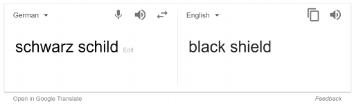
In one of the amazing coincidences of history, “Schwarz” means “black”
in German while “schild” means “shield.” It appears that Karl Schwarzschild
was always destined to discover black holes, even if he himself didn’t
know that.
2.5 Black Holes
Let’s see if we can get an intuitive feel for black holes just by looking
at the Schwarzschild metric. First, note that there is an interesting
length
r
s
= 2GM. (13)
This is the “Schwarzschild radius.” As I’m sure you heard, anything that
enters the Schwarzschild radius, A.K.A. the “event horizon,” cannot ever
escape. Why is that?
16
Note that at r = r
s
, the dt component of the metric becomes 0 and
the dr component becomes infinite. This particular singularity isn’t
“real.” It’s a “coordinate singularity.” There are other coordinates we
could use, like the Kruskal–Szekeres coordinates that do not have this
unattractive feature. We will ignore this.
The more important thing to note is that the dt and dr components
flip signs as r dips below 2GM. This is very significant. Remember that
the flat space metric is
dτ
2
= dt
2
− dx
2
− dy
2
− dz
2
. (14)
The only thing that distinguishes time and space is a sign in the metric!
This sign flips once you cross the event horizon.
Here is why this is important. Say that a massive particle moves a
tiny bit to a nearby space-time point which is separated from the original
point by dτ . If the particle is moving slower than c, then dτ
2
> 0.
However, inside of a black hole, as per Eq. 11, we can see that when
dτ
2
> 0, the particle must either be travelling into the center of the
black hole or away from it. This is just because 11 is of the form
dτ
2
=
(
(+)dt
2
+ (−)dr
2
+ (−)dθ
2
+ (−)dφ
2
if r > 2GM
(−)dt
2
+ (+)dr
2
+ (−)dθ
2
+ (−)dφ
2
if r < 2GM
were (+) denotes a positive quantity and (−) denotes a negative quan-
tity. In order that dτ
2
> 0, we much have dt
2
> 0 outside of the event
horizon but dr
2
> 0 inside the horizon, so dr cannot be 0.
Furthermore, if the particle started outside of the even horizon and
then went in, travelling with dr < 0 along its path, then by continuity
it has no choice but to keep travelling inside with dr < 0 until it hits
the singularity
The reason that a particle cannot “turn around” and leave the black
hole is the exact same reason why you cannot “turn around” and go back
in time. If you think about it, there is a similar “horizon” between you
and your childhood. You can never go back. If you wanted to go back
in time, at some point you would have to travel faster than the speed of
light (faster than 45
◦
).
The r coordinate becomes “time-like” behind the event horizon.
17

Figure 15: Going back in time requires going faster than c, which is
impossible.
Outside of a black hole, we are forced to continue aging and die, t
ever increasing. Inside of a black hole, we would be forced to hit the
singularity and die, r ever decreasing. Death is always gently guiding
us into the future.
Figure 16: Once you have passed the event horizon of a black hole, r
and t “flip,” so now going into the future means going further into the
black hole until you hit the singularity.
2.6 Penrose Diagram for a Black Hole
If we get rid of the angular θ and φ coordinates, our Schwarzschild
space-time only has two coordinates (t, r). Once again, we can cook up
new coordinates that allow us to draw a Penrose diagram. Here is the
result.
18

Figure 17: Penrose diagram of maximally extended space-time with
Schwarzschild metric.
There is a lot to unpack here. Let’s start with the right hand dia-
mond. This is space-time outside of the black hole, where everyone is
safe. The upper triangle is the interior of the black hole. Because the
boundary is a 45
◦
angle, once you enter you cannot leave. This is the
event horizon. The jagged line up top is the singularity that you are
destined to hit once you enter the black hole. From the perspective of
people outside the black hole, it takes an infinite amount of time for
something enter the black hole. It only enters at t = +∞
Figure 18: Penrose diagram of black hole with some lines of constant
r and t labelled.
19

Figure 19: Two worldlines in this space-time, one which enters the
black hole and one which does not.
I’m sure you noticed that there are two other parts to the diagram.
The bottom triangle is the interior of the “white hole” and the left hand
diamond is another universe! This other universe is invisible to the
Schwarzschild coordinates, and only appears once the coordinates are
“maximally extended.”
First let’s look at the white hole. There’s actually nothing too crazy
about it. If something inside the black hole is moving away from the
singularity (with dr > 0) it has no choice but to keep doing so until it
leaves the event horizon. So the stuff that starts in the bottom triangle
is the stuff that comes out of the black hole. (In this context, however,
we call it the white hole). It enters our universe at t = −∞. It is
impossible for someone on the outside to enter the white hole. If they
try, they will only enter the black hole instead. This is because the can’t
go faster than 45
◦
!
Figure 20: Stuff can come out of the white hole and enter our universe
at t = −∞.
20

Okay, now what the hell is up with this other universe? Its exactly
the same as our universe, but different. Note that two people in the
different universes can both enter the black hole and meet inside. How-
ever, they are both doomed to hit the singularity soon after. The two
universes have no way to communicate outside of the black hole.
Figure 21: People from parallel universes can meet inside the black
hole.
But wait! Hold the phone! Black holes exist in real life, right? Is
there a mirror universe on the other side of every black hole????
No. The Schwarzschild metric describes an “eternal black hole” that
has been there since the beginning of time and will be there until the
end of time. Real black holes are not like this. They form when stars
collapse. It is more complicated to figure out what the metric is if you
want to take stellar collapse into account, but it can be done. I will not
write the metric, but I will draw the Penrose diagram.
21

Figure 22: A Penrose diagram for a black hole that forms via stellar
collapse.
Because the black hole forms at a some finite time, there is no white
hole in our Penrose diagram. Likewise, there is no mirror universe.
Its interesting to turn the Penrose diagram upside down, which is
another valid solution to Einstein’s equations. This depicts a universe
in which a white hole has existed since the beginning of the universe. It
keeps spewing out material, getting smaller and smaller, until it disap-
pears at some finite time. No one can enter the white hole. If they try,
they will only see it spew material faster and faster as they get closer.
The white hole will dissolve right before their eyes. That is why they
can’t enter it.
Figure 23: The Penrose diagram for a white hole that exists for some
finite time.
22

2.7 Black Hole Evaporation
I have not mentioned anything about quantum field theory yet, but
I will give you a spoiler: black holes evaporate. This was discovered by
Stephen Hawking in 1975. They radiate energy in the form of very low
energy particles until they do not exist any more. This is a unique fea-
ture of what happens to black holes when you take quantum field theory
into account, and is very surprising. Having said that, this process is
extremely slow. A black hole with the mass of our sun would take 10
67
years to evaporate. Let’s take a look at the Penrose diagram for a black
hole which forms via stellar collapse and then evaporates.
Figure 24: The Penrose diagram for a black hole which forms via stellar
collapse and then evaporates.
23

3 Quantum Field Theory
While reading this section, forget I told you anything about general
relativity. This section only applies to flat Minkowski space and has
nothing to do with black holes.
3.1 Quantum Mechanics
Quantum mechanics is very simple. You only need two things. A
Hilbert space and Hamiltonian. Once you specify those two things, you
are done!
A Hilbert space H is just a complex vector space. States are elements
of the Hilbert space.
|ψi ∈ H. (15)
Our Hilbert space also has a positive definite Hermitian inner product.
hψ|ψi > 0 if |ψi 6= 0. (16)
A Hamiltonian
ˆ
H is just a linear map
ˆ
H = H → H (17)
that is self adjoint.
ˆ
H
†
=
ˆ
H (18)
States evolve in time according to the Schrödinger equation
d
dt
|ψi = −
i
~
ˆ
H |ψi. (19)
Therefore states evolve in time according to
U(t) |ψi ≡ exp
−
i
~
t
ˆ
H
|ψi. (20)
Because
ˆ
H is self adjoint, U(t) is unitary.
U(t)
†
= U(t)
−1
(21)
(Sometimes the Hamiltonian itself depends on time, i.e.
ˆ
H =
ˆ
H(t). In
these cases the situation isn’t so simple.)
I really want to drive this point into your head. Once you have a
Hilbert space H and a Hamiltonian
ˆ
H, you are DONE!
24
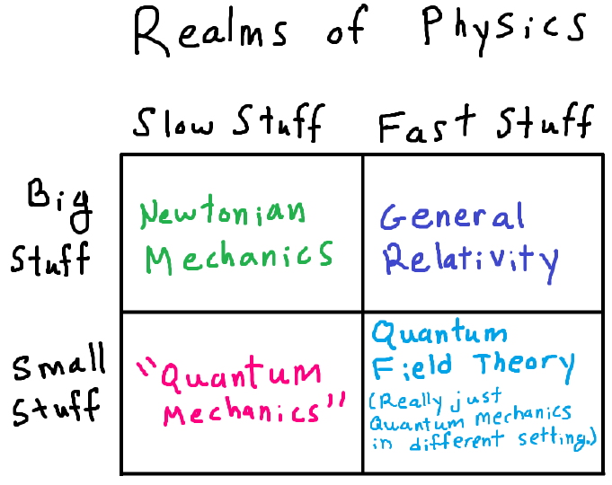
3.2 Quantum Field Theory vs Quantum Mechanics
Different areas of physics need different theories to describe them.
People usually use the term “quantum mechanics” to describe things
that are small but moving very slow. This is the domain of chemistry.
However, once things travel very fast, there is enough energy to make
new particles and destroy old ones. This is the domain of quantum field
theory.
However, mathematically speaking, quantum field theory is just sub-
set of quantum mechanics. States in quantum field theory live in a
Hilbert space and evolve according to a Hamiltonian just like in quan-
tum mechanics.
I am going to be extremely ambitious here and literally just tell you
what this Hilbert space and Hamiltonian actually is for a very simple
quantum field theory. However, I will not describe to you the Hilbert
space of the actual quantum fields we see in real life like the photon
field, the electron field, etc. Actual particles have a confusing property
called “spin” which I don’t want to get into. I will instead tell you
about the quantum field theory of a fictitious “spin 0” particle that could
theoretically exist in real life but doesn’t appear to. Furthermore, this
particle will not “interact” with any other particle, making its analysis
particularly simple.
25

3.3 The Hilbert Space of QFT: Wavefunctionals
A classical field is a function φ(x) from space into R.
φ : R
3
→ R. (22)
We denote the space of smooth functions on R
3
by C
∞
(R
3
).
φ ∈ C
∞
(R
3
). (23)
Each particular φ is called a “classical field configuration.” Each value
φ(x) for some particular x is called a “field variable.”
Figure 25: A classical field assigns a real number to each point in
space. I have suppressed the three spatial dimensions into just one, x,
for simplicity.
Now I’m going to tell you what a quantum field state is. Are you
ready? A quantum field state is a functional from classical fields to
complex numbers.
Ψ : C
∞
(R
3
) → C (24)
H
QFT
= all such wave functionals (25)
These are called “wave functionals.” Let’s say you have two wave func-
tionals Ψ and Φ. The inner product is this infinite dimensional integral,
which integrates over all possible classical field configurations:
hΨ|Φi =
Z
Y
x∈R
3
dφ(x)
Ψ[φ]
∗
Φ[φ]
. (26)
Obviously, the product over x ∈ R
3
isn’t mathematically well defined.
However, there’s a whole branch of physics called “lattice field theory”
where people discretize space into lattices in order to compute things
26
on a super computer. Furthermore, physicists have many reasons to
believe that if we had a full theory of quantum gravity, we would realize
that quantum field theory as we know it does break down at very tiny
Planck-length sized distances. Most likely it would not be anything as
crude as a literal lattice, but something must be going on at really small
lengths. Anyway, because we don’t have a theory of quantum gravity,
this is the best we can do for now.
The physical interpretation is that if |Ψ[φ]|
2
is very big for a partic-
ular φ, then the quantum field is very likely to “be” in the classical field
configuration φ.
Note that we have a basis of wave functionals given by
Ψ
φ
0
[φ] ∝
(
1 if φ = φ
0
0 if φ 6= φ
0
(27)
for all φ
0
∈ C
∞
(R
3
). We can write them as
|Ψ
φ
0
i
(You should think of these as the i in |ii. Each classical field φ
0
labels
a “coordinate” of the QFT Hilbert space.) All other wave functionals
can be written as a linear combination of these wave functionals with
complex coefficients. However, this basis of the Hilbert space is physi-
cally useless. You would never ever see a quantum field state like these
in real life. (The reason is that they have infinite energy.) I will tell you
about a more useful basis for quantum field states a bit later.
3.4 Two Observables
An observable
ˆ
O is a linear map
ˆ
O : H → H (28)
that is self adjoint
ˆ
O
†
=
ˆ
O. (29)
Because it is self adjoint, all of its eigenvalues must be real numbers.
An eigenstate |ψi of
ˆ
O that satisfies
ˆ
O|ψi = λ |ψi (30)
for some λ ∈ R has the interpretation of having definite value λ under
the measurement corresponding to
ˆ
O.
27

There are two important sets of observables I have to tell you about
for these wave functionals. They are called
ˆ
φ(x) and ˆπ(x). (31)
There are an infinite number of them, one for each x. You should think
of the measurements
ˆ
φ(x) and ˆπ(x) as measurements occurring at the
point x in space. They are linear operators
ˆ
φ(x) : H
QFT
→ H
QFT
and ˆπ(x) : H
QFT
→ H
QFT
which are defined as follows.
ˆ
φ(x)Ψ
[φ] ≡ φ(x)Ψ[φ] (32)
ˆπ(x)Ψ
[φ] ≡
~
i
δ
δφ(x)
Ψ[φ] (33)
(Use the hats to help you!
ˆ
φ(x) is an operator acting on wave function-
als, while φ is the classical field configuration at which we are evaluating
our wave-functional. φ(x) is just the value of that input φ at x.)
First let’s talk about
ˆ
φ(x). It is the observable that “measures the
value of the field at x.” For example, the expected field value at x would
be
hΨ|
ˆ
φ(x) |Ψi =
Z
Y
x
0
∈R
3
dφ(x
0
)|Ψ[φ]|
2
φ(x).
Note that our previously defined Ψ
φ
0
are eigenstates of this operator.
For any φ
0
∈ C
∞
(R
3
), we have
ˆ
φ(x) |Ψ
φ
0
i = φ
0
(x) |Ψ
φ
0
i. (34)
The physical interpretation of ˆπ(x) is a bit obscure. First off, if you
don’t know,
δ
δφ(x)
(35)
is called the “functional derivative.” It is defined by
δφ(x)
δφ(y)
≡ δ
3
(x − y ). (36)
(δ
3
(x − y) is the three dimensional Dirac delta function. It satisfied
R
d
3
xf(x)δ
3
(x − y) = f(y) for any f : R
3
→ C, where d
3
x = dxdydz
28

is the three dimensional volume measure.) This is just the infinite di-
mensional version of the partial derivative in multivariable calculus.
∂x
i
∂x
j
= δ
ij
. (37)
Basically, ˆπ(x) measures the rate of change of the wave functional with
respect to one particular field variable φ(x). (The i is there to make it
self-adjoint.) I don’t want to get bogged down in its physical interpre-
tation.
3.5 The Hamiltonian
Okay, I’ve now told you about the Hilbert space, the inner prod-
uct, and a few select observables. Now I’m going to tell you what the
Hamiltonian is and then I’ll be done!
ˆ
H =
1
2
Z
d
3
x
ˆπ
2
+ (∇
ˆ
φ)
2
+ m
2
ˆ
φ
2
(38)
Done! (Here m is just a real number.)
(Now you might be wondering where I got this Hamiltonian from.
The beautiful thing is, I do not have to tell you! I am just telling
you the laws. Nobody truly knows where the laws of physics come
from. The best we can hope for is to know them, and then derive
their consequences. Now obviously I am being a bit cheeky, and there
are many desirable things about this Hamiltonian. But you shouldn’t
worry about that at this stage.)
I used some notation above that I have not defined. I am integrating
over all of space, so really I should have written ˆπ(x) and
ˆ
φ(x) but I
suppressed that dependence for aesthetics. Furthermore, that gradient
term needs to be written out explicitly.
(∇
ˆ
φ)
2
=
∂
x
ˆ
φ
2
+
∂
y
ˆ
φ
2
+
∂
z
ˆ
φ
2
where
∂
x
ˆ
φ(x, y, z) = lim
∆x→0
ˆ
φ(x + ∆x, y, z) −
ˆ
φ(x, y, z)
∆x
.
Let’s get an intuitive understanding for this Hamiltonian by looking at
it term by term.
The
ˆπ(x)
2
29

term means that a wavefunctional has a lot of energy if it changes quickly
when a particular field variable is varied.
For the other two terms, let’s imagine that our fields are well ap-
proximated by the state Ψ
φ
0
, i.e. it is one of those basis states we talked
about previously. This means it is “close” to being a “classical” field.
|Ψi ≈ |Ψ
φ
0
i. (39)
Then the
(∇
ˆ
φ)
2
term means that a wavefunctional has a lot of energy if φ
0
has a big
gradient. Similarly, the
m
2
ˆ
φ
2
term means the wave functional has a lot of energy if φ
0
is non-zero in
a lot of places.
3.6 The Ground State
I will now tell you what the lowest energy eigenstate of this Hamil-
tonian is. It is
Ψ
0
[φ] ∝ exp
−
1
2~
Z
d
3
k
p
k
2
+ m
2
|φ
k
|
2
(40)
where
φ
k
≡
Z
d
3
x
(2π)
3/2
φ(x)e
−ik·x
(41)
are the Fourier components (or “modes”) of the classical field config-
uration φ(x). Because φ is real, φ
∗
k
= φ
−k
. Note d
3
k is the three-
dimensional volume measure over k-space, and k
2
= |k|
2
. The bigger
|k| is, the higher the “frequency” of the Fourier mode is.
Let’s try and understand this wave functional qualitatively. It takes
its largest value when φ(x) = 0. The larger the Fourier components
of the classical field, the smaller Ψ
0
is. Therefore the wave functional
outputs very tiny number for classical fields that are far from 0. Fur-
thermore, because of the
√
k
2
+ m
2
term, the high frequency Fourier
components are penalized more heavily that the low frequency Fourier
components. Therefore, the wave functional Ψ
0
is very small for big
and jittery classical fields, and very large for small and gradually vary-
ing classical fields.
30

Figure 26: Some sample classical field configurations and the relative
size of Ψ
0
when evaluated at each one. The upper-left field maximizes
Ψ
0
because it is 0. The upper-right field is pretty close to 0, so Ψ
0
is
still pretty big. The lower-left field makes Ψ
0
small because it contains
large field values. The lower-right field makes Ψ
0
because its frequency
|k| is large even though the Fourier-coefficient is not that large.
First, let’s recall what we mean by ground state. Because |Ψ
0
i is an
energy eigenstate,
ˆ
H |Ψ
0
i = E
0
|Ψ
0
i (42)
for some energy E
0
. However, any other energy eigenstate will neces-
sarily have an eigenvalue that is bigger than E
0
.
Intuitively speaking, why is |Ψ
0
i the ground state? It’s because it
negotiates all of the competing interests of the terms in the Hamiltonian
to minimize it’s eigenvalue. Recall that there are three terms in the
Hamiltonian from Eq. 38. Let’s go through all three terms how see how
Ψ
0
tries to minimize each one.
1. The ˆπ
2
term doesn’t want the functional to vary too quickly as
the classical field input is changed. This is minimized because Ψ
0
varies like a Gaussian in terms of the Fourier components φ
k
.
2. The (∇
ˆ
φ)
2
term is minimized when likely classical field config-
urations have small gradients. This is minimized because of the
√
k
2
+ m
2
factor, which penalizes high-gradient jittery fields more
harshly than small-gradient gradually varying fields.
31

3. The m
2
φ
2
term wants likely classical field configurations to have
field values φ(x) close to 0. This is minimized by making Ψ
0
peak
around the classical field configuration φ(x) = 0.
Now that we have some appreciation for the ground state, I want to
rewrite it in a suggestive way:
Ψ
0
[φ] ∝ exp
−
1
2~
Z
d
3
k
p
k
2
+ m
2
|φ
k
|
2
∝
Y
k∈R
3
exp
−
1
2~
p
k
2
+ m
2
|φ
k
|
2
.
We can see that |Ψ
0
i “factorizes” nicely when written in terms of the
Fourier components φ
k
of the classical field input.
3.7 Particles
You ask, “Alright, great, I can see what a quantum field is. But what
does this have to do with particles?”
Great question. These wave functionals seem to have nothing to do
with particles. However, the particle states are hiding in these wave
functionals, somehow. It turns out that we can make wave functionals
that describe a state with a certain number of particles possessing some
specified momenta ~k. Here is how you do it:
Let’s say that for each k, there are n
k
particles present with momenta
~k. Schematically, the wavefunctionals corresponding to these states are
Ψ[φ] ∝
Y
k∈R
3
F
n
k
(φ
k
, φ
−k
) exp
−
1
2~
p
k
2
+ m
2
|φ
k
|
2
. (43)
for some set of functions F
n
k
.
However, people never really work in terms of these functions F
n
k
,
whatever they are. More commonly, states are written in terms of “oc-
cupation number” notation. We would the write state in Eq. 43 as
|Ψi = |n
k
1
, n
k
2
, n
k
3
, . . .i. (44)
These states are definite energy states because they are eigenstates of
the Hamiltonian.
ˆ
H |n
k
1
, n
k
2
, n
k
3
, . . .i =
E
0
+
X
k∈R
2
n
k
p
~
2
k
2
+ m
2
|n
k
1
, n
k
2
, n
k
3
, . . .i
(45)
32

(Remember that E
0
is the energy of the ground state |Ψ
0
i.) If you ever
took a class in special relativity, you would have learned that the energy
E of a particle with momentum ~p and mass m is equal to
E
2
= p
2
c
2
+ m
2
c
4
. (46)
That is exactly where that comes from! (Remember we set c = 1.)
This is exactly the energy for a collection of particles with mass m and
momentum ~k! The ground state is just the state when all n
k
= 0.
Not every state can be written in the form of Eq. 44. However,
every state can be written in terms of a linear combination of states
of that form. Therefore, we now have two different ways to understand
the Hilbert space of quantum field theory. On one hand, we can think
of them as wave functionals. On the other hand, we can think of them
in terms of particle occupation numbers. These are really two different
bases for the same Hilbert space.
There’s something I need to point out. These particle states I’ve
written are completely “delocalized” over all of space. These particles
do not exist at any particular location. They are infinite plane waves
spread out over the whole universe. This is because they are energy (and
momentum) eigenstates, meaning they have a well-defined energy. If we
wanted to “localize” these particles, we could make a linear combination
of particles of slightly different momenta in order to make a Gaussain
wave packet. This Gaussian wave packet would not have a perfectly well
defined energy or momentum, though. There would be some uncertainty
because it is a superposition of energy eigenstates.
So if we momentarily call |ki to be the state containing just one
particle with momentum k, then particle state which is a wavepacket of
momentum k
0
and frequency width σ could be written as
|k
0
i
Gaussian
∝
Z
d
3
k exp
−
(k−k
0
)
2
2σ
2
|ki.
I have included a picture of a wavepacket in the image below. However,
don’t forget that our QFT “wavepacket” is really a complicated wave
functional, and does not have any interpretation as a classical field.
33

Figure 27: A localized wave packet is the sum of completely delocalized
definite-frequency waves. Note that you can’t localize a wave packet into
a volume that isn’t at least a few times as big as its wavelength.
There’s four final things you might be wondering about particles.
Firstly, where are the “anti-particles” you’ve heard so much about? The
answer is that there are no anti-particles in the quantum field I’ve de-
scribed here. This is because the classical field configurations are func-
tions φ : R
3
→ R. If our classical fields were functions φ : R
3
→ C,
then we would find that there are two types of particles, one of which we
would call “anti particles.” Secondly, I should say that the particles I’ve
described are bosons. That means we can have as many particles as we
want with some momentum ~k. In other words, our occupation num-
bers can be any positive integer. A fermionic field is different. Fermionic
fields can only have occupation numbers of 0 or 1, so they are rather “dig-
ital” in that sense. Fermionic quantum field states therefore do not have
the nice wavefunctional interpretation that bosonic quantum fields have.
Thirdly, the particle we’ve constructed here has no spin, i.e. it is a “spin
0” particle. The sorts of particles we’re most used to, like electrons and
photons, are not of this type. They have spin
1
2
and spin 1, respectively.
Fourthly, where are the Feynman diagrams you’ve probably heard so
much about? Feynman diagrams are useful for describing particle in-
teractions. For example, an electron can emit or absorb a photon, so we
say the electron field interacts with the photon field. I have only told
you here about non-interacting particles, which is perfectly sufficient for
our purposes. Feynman diagrams are often used to compute “scattering
amplitudes.” For example, say I send in two electron wave packets into
each other with some momenta and relative angles, wait a while, and
then observe two electrons wave packets leaving with new momenta at
different relative angles. Physicists use Feynman diagrams as a tool in
34

order to calculate what the probability of such an event is.
3.8 Entanglement properties of the ground state
We have now looked out our Hilbert space H
QFT
in two different
bases: the wavefunctional basis and the particle basis. Both have their
strengths and weaknesses. However, I would like to bring up something
interesting. Thinking in terms of the wavefunctional basis, we can see
that H
QFT
can be decomposed into a tensor product of Hilbert spaces,
one for each position x in space.
H
QFT
=
O
x∈R
3
H
x
(47)
(Once again, we might imagine that our tensor product is not truly taken
over all of R
3
, but perhaps over a lattice of Planck-length spacing, for
all we know.) Each local Hilbert space H
x
is given by all normalizable
functions from R → C. Following mathematicians, we might call such
functions L
2
(R).
H
x
= L
2
(R)
Fixing x, each state in H
x
simply assigns a complex number to each
possible classical value of φ(x). Once we tensor together all H
x
, we
recover our space of field wave functionals. The question I now ask you
is: what are the position-space entanglement properties of the ground
state?
Let’s back up a bit and remind ourselves what the ground state
again. We wrote it in terms of the Fourier components:
Ψ
0
[φ] ∝ exp
−
1
2~
Z
d
3
k
p
k
2
+ m
2
|φ
k
|
2
φ
k
≡
Z
d
3
x
(2π)
3/2
φ(x)e
−ik·x
We can plug in the bottom expression into the top expression to express
Ψ
0
[φ] in terms of the position space classical field φ(x).
Ψ
0
[φ] ∝ exp
−
1
2~
ZZZ
d
3
k
d
3
xd
3
y
(2π)
3
e
−ik·(x−y)
p
k
2
+ m
2
φ(x)φ(y)
∝ exp
−
1
2~
ZZ
d
3
xd
3
y
(2π)
3
f(|x − y|)φ(x)φ(y)
35
One could in principle perform the k integral to compute f(|x − y|),
although I won’t do that here. (There’s actually a bit of funny business
you have to do, introducing a “regulator” to make the integral converge.)
The important thing to note is that the values of the field variables φ(x)
and φ(y) are entangled together by f(|x −y |), and the wave functional
Ψ
0
does not factorize nicely in position space the way it did in Fourier
space. The bigger f(|x−y|) is, the larger the entanglement between H
x
and H
y
is. We can see that in the ground state, the value of the field at
one point is quite entangled with the field at other points. Indeed, there
is a lot of short-range entanglement all throughout the universe. How-
ever, it turns out that f(|x −y|) becomes very small at large distances.
Therefore, nearby field variables are highly entangled, while distant field
variables are not very entangled.
This is not such a mysterious property. If your quantum field is in
the ground state, and you measure the value of the field at some x to
be φ(x) then all this means is that nearby field values are likely to also
be close to φ(x). This is just because the ground state wave functional
is biggest for classical fields that vary slowly in space.
You might wonder if this entanglement somehow violates causality.
Long story short, it doesn’t. This entanglement can’t be used to send
information faster than light. (However, it does have some unintuitive
consequences, such as the Reeh–Schlieder theorem.)
Let me wrap this up by saying what this has to do with the Firewall
paradox. Remember, in this section we have only discussed QFT in flat
space! However, while the space-time at the horizon of a black hole is
curved, it isn’t curved that much. Locally, it looks pretty flat. There-
fore, one would expect for quantum fields in the vicinity of the horizon
to behave much like they would in flat space. This means that low en-
ergy quantum field states will still have a strong amount of short-range
entanglement because short-range entanglement lowers the energy of the
state. (This is because of the (∇
ˆ
φ)
2
term in the Hamiltonian.) However,
the Firewall paradox uses the existence of this entanglement across the
horizon to make a contradiction. One resolution to the contradiction is
to say that there’s absolutely no entanglement across the horizon what-
soever. This would mean that there is an infinite energy density at the
horizon, contradicting the assumption that nothing particularly special
happens there.
36

4 Statistical Mechanics
4.1 Entropy
Statistical Mechanics is a branch of physics that pervades all other
branches. Statistical mechanics is relevant to Newtonian mechanics,
relativity, quantum mechanics, and quantum field theory.
Figure 28: Statistical mechanics applies to all realms of physics.
Its exact incarnation is a little different in each quadrant, but the
basic details are identical.
The most important quantity in statistical mechanics is called “en-
tropy,” which we label by S. People sometimes say that entropy is a
measure of the “disorder” of a system, but I don’t think this a good way
to think about it. But before we define entropy, we need to discuss two
different notions of state: “microstates” and “macrostates.”
In physics, we like to describe the real world as mathematical objects.
In classical physics, states are points in a “phase space.” Say for example
you had N particles moving around in 3 dimensions. It would take 6N
real numbers to specify the physical state of this system at a given
instant: 3 numbers for each particle’s position and 3 numbers for each
particle’s momentum. The phase space for this system would therefore
just be R
6N
.
(x
1
, y
1
, z
1
, p
x
1
, p
y
1
, p
z
1
, . . . x
N
, y
N
, z
N
, p
x
N
, p
y
N
, p
z
N
) ∈ R
6N
(In quantum mechanics, states are vectors in a Hilbert space H instead
of points in a phase space. We’ll return to the quantum case a bit later.)
37

A “microstate” is a state of the above form. It contains absolutely
all the physical information that an omniscent observer could know. If
you were to know the exact microstate of a system and knew all of the
laws of physics, you could in principle deduce what the microstate will
be at all future times and what the microstate was at all past times.
However, practically speaking, we can never know the true microstate
of a system. For example, you could never know the positions and mo-
menta of every damn particle in a box of gas. The only things we can
actually measure are macroscopic variables such as internal energy, vol-
ume, and particle number (U, V, N). A “macrostate” is just a set of
microstates. For examples, the “macrostate” of a box of gas labelled by
(U, V, N) would be the set of all microstates with energy U, volume V ,
and particle number N. The idea is that if you know what macrostate
your system is in, you know that your system is equally likely to truly
be in any of the microstates it contains.
Figure 29: You may know the macrostate, but only God knows the
microstate.
I am now ready to define what entropy is. Entropy is a quantity asso-
38

ciated with a macrostate. If a macrostate is just a set of Ω microstates,
then the entropy S of the system is
S ≡ k log Ω. (48)
Here, k is Boltzmann’s constant. It is a physical constant with units of
energy / temperature.
k ≡ 1.38065 × 10
−23
Joules
Kelvin
(49)
The only reason that we need k to define S is because the human race
defined units of temperature before they defined entropy. (We’ll see
how temperature factors into any of this soon.) Otherwise, we probably
would have set k = 1 and temperature would have the same units as
energy.
You might be wondering how we actually count Ω. As you probably
noticed, the phase space R
6N
is not discrete. In that situation, we
integrate over a phase space volume with the measure
d
3
x
1
d
3
p
1
. . . d
3
x
N
d
3
p
N
.
However, this isn’t completely satisfactory because position and mo-
mentum are dimensionful quantities while Ω should be a dimensionless
number. We should therefore divide by a constant with units of posi-
tion times momentum. Notice, however, that because S only depends
on log Ω, any constant rescaling of Ω will only alter S by a constant and
will therefore never affect the change in entropy ∆S of some process. So
while we have to divide by a constant, whichever constant we divide by
doesn’t affect the physics.
Anyway, even though we are free to choose whatever dimensionful
constant we want, the “best” is actually Planck’s constant h! Therefore,
for a classical macrostate that occupies a phase space volume Vol,
Ω =
1
N!
1
h
3N
Z
Vol
N
Y
i=1
d
3
x
i
d
3
p
i
. (50)
(The prefactor 1/N! is necessary if all N particles are indistinguishable.
It is the cause of some philosophical consternation but I don’t want to
get into any of that.)
Let me now explain why I think saying entropy is “disorder” is not
such a good idea. Different observers might describe reality with differ-
ent macrostates. For example, say your room is very messy and disor-
ganized. This isn’t a problem for you, because you spend a lot of time
39

in there and know where everything is. Therefore, the macrostate you
use to describe your room contains very few microstates and has a small
entropy. However, according to your mother who has not studied your
room very carefully, the entropy of your room is very large. The point
is that while everyone might agree your room is messy, the entropy of
your room really depends on how little you know about it.
4.2 Temperature and Equilibrium
Let’s say we label our macrostates by their total internal energy
U and some other macroscopic variables like V and N. (Obviously,
these other macroscopic variables V and N can be replaced by different
quantities in different situations, but let’s just stick with this for now.)
Our entropy S depends on all of these variables.
S = S(U, V, N) (51)
The temperature T of the (U, V, N) macrostate is then be defined to be
1
T
≡
∂S
∂U
V,N
. (52)
The partial derivative above means that we just differentiate S(U, V, N)
with respect to U while keeping V and N fixed.
If your system has a high temperature and you add a bit of energy
dU to it, then the entropy S will not change much. If your system has a
small temperature and you add a bit of energy, the entropy will increase
a lot.
Next, say you have two systems A and B which are free to trade
energy back and forth.
Figure 30: Two systems A and B trading energy. U
A
+ U
B
is fixed.
40

Say system A could be in one of Ω
A
possible microstates and system
B could be in Ω
B
possible microstates. Therefore, the total AB system
could be in Ω
A
Ω
B
possible microstates. Therefore, the entropy S
AB
of
both systems combined is just the sum of entropies of both sub-systems.
S
AB
= k log(Ω
A
Ω
B
) = k log Ω
A
+ k log Ω
B
= S
A
+ S
B
(53)
The crucial realization of statistical mechanics is that, all else being
equal, a system is most likely to find itself in a macrostate corresponding
to the largest number of microstates. This is the so-called “Second law
of thermodynamics”: for all practical intents and purposes, the entropy
of a closed system always increases over time. It is not really a physical
“law” in the regular sense, it is more like a profound realization.
Therefore, the entropy S
AB
of our joint AB system will increase as
time goes on until it reaches its maximum possible value. In other words,
A and B trade energy in a seemingly random fashion that increases S
AB
on average. When S
AB
is finally maximized, we say that our systems
are in “thermal equilibrium.”
Figure 31: S
AB
is maximized when U
A
has some particular value.
(It should be noted that there will actually be tiny random "thermal"
fluctuations around this maximum.)
Let’s say that the internal energy of system A is U
A
and the internal
energy of system B is U
B
. Crucially, note that the total energy of
combined system
U
AB
= U
A
+ U
B
is constant over time! This is because energy of the total system is
conserved. Therefore,
dU
A
= −dU
B
.
41

Now, the combined system will maximize its entropy when U
A
and U
B
have some particular values. Knowing the value of U
A
is enough though,
because U
B
= U
AB
− U
A
. Therefore, entropy is maximized when
0 =
∂S
AB
∂U
A
. (54)
However, we can rewrite this as
0 =
∂S
AB
∂U
A
=
∂S
A
∂U
A
+
∂S
B
∂U
A
=
∂S
A
∂U
A
−
∂S
B
∂U
B
=
1
T
A
−
1
T
B
.
Therefore, our two systems are in equilibrium if they have the same
temperature!
T
A
= T
B
(55)
If there are other macroscopic variables we are using to define our
macrostates, like volume V or particle number N, then there will be
other quantities that must be equal in equibrium, assuming our two sys-
tems compete for volume or trade particles back and forth. In these
cases, we define the quantities P and µ to be
P
T
≡
∂S
∂V
U,N
µ
T
≡ −
∂S
∂N
U,V
. (56)
P is called “pressure” and µ is called “chemical potential.” In equilib-
rium, we would also have
P
A
= P
B
µ
A
= µ
B
. (57)
(You might object that pressure has another definition, namely force di-
vided by area. It would be incumbent on us to check that this definition
matches that definition in the relevant situation where both definitions
have meaning. Thankfully it does.)
42

4.3 The Partition Function
Figure 32: If you want to do statistical mechanics, you really should
know about the partition function.
Explicitly calculating Ω for a given macrostate is usually very hard.
Practically speaking, it can only be done for simple systems you under-
stand very well. However, physicists have developed an extremely pow-
erful way of doing statistical mechanics even for complicated systems.
It turns out that there is a function of temperature called the “partition
function” that contains all the information you’d care to know about
your macrostate when you are working in the “thermodynamic limit.”
This function is denoted Z(T ). Once you compute Z(T ) (which is usu-
ally much easier than computing Ω) it is a simple matter to extract the
relevant physics.
Before defining the partition function, I would like to talk a bit about
heat baths. Say you have some system S in a very large environment E.
Say you can measure the macroscopic variables of S, including its energy
E at any given moment. (We use E here to denotes energy instead of
U when talking about the partition function.) The question I ask is: if
the total system has a temperature T , what’s the probability that S has
some particular energy E?
43

Figure 33: A large environment E and system S have a fixed total en-
ergy E
tot
. E is called a “heat bath” because it is very big. The combined
system has a temperature T .
We should be picturing that S and E are evolving in some compli-
cated way we can’t understand. However, their total energy
E
tot
= E + E
E
(58)
is conserved. We now define
Ω
S
(E) ≡ num. microstates of S with energy E (59)
Ω
E
(E
E
) ≡ num. microstates of E with energy E
E
.
Therefore, the probability that S has some energy E is proportional
to the number of microstates where S has energy E and E has energy
E
tot
− E.
Prob(E) ∝ Ω
S
(E)Ω
E
(E
tot
− E) (60)
Here is the important part. Say that our heat bath has a lot of energy:
E
tot
E. As far as the heat bath is concerned, E is a very small
amount of energy. Therefore,
Ω
E
(E
tot
− E) = exp
1
k
S
E
(E
tot
− E)
≈ exp
1
k
S
E
(E
tot
) −
E
kT
by Taylor expanding S
E
in E and using the definition of temperature.
We now have
Prob(E) ∝ Ω
S
(E) exp
−
E
kT
.
44

Ω
S
(E) is sometimes called the “degeneracy” of E. In any case, we can
easily see what the ratio of Prob(E
1
) and Prob(E
2
) must be.
Prob(E
1
)
Prob(E
2
)
=
Ω
S
(E
1
)e
−E
1
/kT
Ω
S
(E
2
)e
−E
2
/kT
Furthermore, we can use the fact that all probabilities must sum to 1 in
order to calculate the absolute probability. We define
Z(T ) ≡
X
E
Ω
S
(E)e
−E/kT
(61)
=
X
s
e
−E
s
/kT
where
P
s
is a sum over all states of S. Finally, we have
Prob(E) =
Ω
S
(E)e
−E/kT
Z(T )
(62)
However, more than being a mere proportionality factor, Z(T ) takes
on a life of its own, so it is given the special name of the “partition
function.” Interestingly, Z(T ) is a function that depends on T and
not E. It is not a function that has anything to do with a particular
macrostate. Rather, it is a function that has to with every microstate
at some temperature. Oftentimes, we also define
β ≡
1
kT
and write
Z(β) =
X
s
e
−βE
s
. (63)
The partition function Z(β) has many amazing properties. For one,
it can be used to write an endless number of clever identities. Here is
one. Say you want to compute the expected energy hEi your system
has at temperature T .
hEi =
X
s
E
s
Prob(E
s
)
=
P
s
E
s
e
−βE
s
Z(β)
= −
1
Z
∂
∂β
Z
= −
∂
∂β
log Z
45

This expresses the expected energy hEi as a function of temperature.
(We could also calculate hE
n
i for any n if we wanted to.)
Where the partition function really shines is in the “thermodynamic
limit.” Usually, people define the thermodynamic limit as
N → ∞ (thermodynamic limit) (64)
where N is the number of particles. However, sometimes you might
be interested in more abstract systems like a spin chain (the so-called
“Ising model”) or something else. There are no “particles” in such a
system, however there is still something you would justifiably call the
thermodynamic limit. This would be when the number of sites in your
spin chain becomes very large. So N should really just be thought of
as the number of variables you need to specify a microstate. When
someone is “working in the thermodynamic limit,” it just means that
they are considering very “big” systems.
Of course, in real life N is never infinite. However, I think we can
all agree that 10
23
is close enough to infinity for all practical purposes.
Whenever an equation is true “in the thermodynamic limit,” you can
imagine that there are extra terms of order
1
N
unwritten in your equation
and laugh at them.
What is special about the thermodynamic limit is that Ω
S
becomes,
like, really big...
Ω
S
= (something)
N
Furthermore, the entropy and energy will scale with N
S
S
= NS
1
E = NE
1
In the above equation, S
1
and E
1
can be thought of as the average
amount of entropy per particle.
Therefore, we can rewrite
Prob(E) ∝ Ω
S
(E) exp
−
1
kT
E
= exp
1
k
S
S
−
1
kT
E
= exp
N
1
k
S
1
−
1
kT
E
1
.
The thing to really gawk at in the above equation is that the probability
that S has some energy E is given by
Prob(E) ∝ e
N(...)
.
I want you to appreciate how insanely big e
N(...)
is in the thermody-
namic limit. Furthermore, if there is even a miniscule change in (. . .),
46

Prob(E) will change radically. Therefore, Prob(E) will be extremely
concentrated at some particular energy, and deviating slightly from that
maximum will cause Prob(E) to plummit.
Figure 34: In the thermodynamic limit, the system S will have a well
defined energy.
We can therefore see that if the energy U maximizes Prob(E), we
will essentially have
Prob(E) ≈
(
1 if E = U
0 if E 6= U
.
Let’s now think back to our previously derived equation
hEi = −
∂
∂β
log Z(β).
Recall that hEi is the expected energy of S when it is coupled to a heat
bath at some temperature. The beauty is that in the thermodynamic
limit where our system S becomes very large, we don’t even have to
think about the heat bath anymore! Our system S is basically just in
the macrostate where all microstates with energy U are equally likely.
Therefore,
hEi = U (thermodynamic limit)
and
U = −
∂
∂β
log Z(β) (65)
is an exact equation in the thermodynamic limit.
47

Let’s just appreciate this for a second. Our original definition of
S(U) was
S(U) = k log(Ω(U))
and our original definition of temperature was
1
T
=
∂S
∂U
.
In other words, T is a function of U. However, we totally reversed logic
when we coupled our system to a larger environment. We no longer
knew what the exact energy of our system was. I am now telling you
that instead of calculating T as a function of U, when N is large we are
actually able to calculate U as a function of T ! Therefore, instead of
having to calculate Ω(U), we can just calculate Z(T ) instead.
I should stress, however, that Z(T ) is still a perfectly worthwhile
thing to calculate even when your system S isn’t “big.” It will still give
you the exact average energy hEi when your system is in equilibrium
with a bigger environment at some temperature. What’s special about
the thermodynamic limit is that you no longer have to imagine the heat
bath is there in order to interpret your results, because any “average
quantity” will basically just be an actual, sharply defined, “quantity.” In
short,
Z(β) = Ω(U)e
−βU
(thermodynamic limit) (66)
It’s worth mentioning that the other contributions to Z(β) will also be
absolute huge; they just won’t be as stupendously huge as the term due
to U.
Okay, enough adulation for the partition function. Let’s do some-
thing with it again. Using the above equation there is a very easy way
to figure out what S
S
(U) is in terms of Z(β).
S
S
(U) = k log Ω
S
(U)
= k log
Ze
βU
(thermodynamic limit)
= k log Z + kβU
= k
1 − β
∂
∂β
log Z
(Gah. Another amazing identity, all thanks to the partition function.)
This game that we played, coupling our system S to a heat bath so
we could calculate U as a function of T instead of T as a function of
U, can be replicated with other quantities like the chemical potential µ
(defined in Eq. 57). We could now imagine that S is trading particles
48

with a larger environment. Our partition function would then be a
function of µ in addition to T .
Z = Z(µ, T )
In the thermodynamic limit, we could once again use our old tricks to
find N in terms of µ.
4.4 Free energy
Now that we’re on an unstoppable victory march of introductory
statistical mechanics, I think I should define a quantity closely related
to the partition function: the “free energy” F .
F ≡ U − TS (67)
(This is also called the “Helmholtz Free Energy.”) F is defined for any
system with some well defined internal energy U and entropy S when
present in a larger environment which has temperature T . Crucially,
the system does not need to be in thermal equilibrium with the environ-
ment. In other words, free energy is a quantity associated with some
system which may or may not be in equilibrium with an environment at
temperature T .
Figure 35: A system with internal energy U and entropy S in a heat
bath at temperature T has free energy F = U − T S.
Okay. So why did we define this quantity F ? The hint is in the
name “free energy.” Over time, the system will equilibriate with the
environment in order to maximize the entropy of the whole world. While
doing so, the energy U of the system will change. So if we cleverly leave
our system in a larger environment, under the right circumstances we
49

can let the second law of thermodynamics to do all the hard work,
transferring energy into our system at no cost to us! I should warn
you that ∆F is actually not equal to the change in internal energy ∆U
that occurs during this equilibriation. This is apparent just from its
definition. (Although it does turn out that F is equal to the “useful
work” you can extract from such a system.)
The reason I’m telling you about F is because it is a useful quan-
tity for determining what will happen to a system at temperature T .
Namely, in the thermodynamic limit, the system will minimize F by
equilibriating with the environment.
Recall Eq. 66 (reproduced below).
Z(β) = Ω(U)e
−βU
(thermodynamic limit)
If our system S is in equilibrium with the heat bath, then
Z(β) = exp
1
k
S − βU
(at equilibrium in thermodynamic limit)
= exp(−βF ).
First off, we just derived another amazing identity of the partition func-
tion. More importantly, recall that U, as written in Eq. 66, is defined
to be the energy that maximizes Ω(U)e
−βU
, A.K.A. the energy that
maximizes the entropy of the world. Because we know that the entropy
of the world always wants to be maximized, we can clearly see that F
wants to be minimized, as claimed.
Therefore, F is a very useful quantity! It always wants to be min-
imized at equilibrium. It can therefore be used to detect interesting
phenomena, such as phase transitions.
4.5 Phase Transitions
Let’s back up a bit and think about a picture we drew, Fig. 34. It’s
a very suggestive picture that begs a very interesting question. What
if, at some critical temperature T
c
, a new peak grows and overtakes our
first peak?
50

Figure 36: A phase transition, right below the critical temperature T
c
,
at T
c
, and right above T
c
.
This can indeed happen, and is in fact what a physicist would call a
“first order phase transition.” We can see that will be a discontinuity in
the first derivative of Z(T ) at T
c
. You might be wondering how this is
possible, given the fact that from its definition, Z is clearly an analytic
function as it is a sum of analytic functions. The thing to remember is
that we are using the thermodynamic limit, and the sum of an infinite
number of analytic functions may not be analytic.
Because there is a discontinuity in the first derivative of Z(β), there
will be a discontinuity in E = −
∂
∂β
log Z. This is just the “latent heat”
you learned about in high school. In real life systems, it takes some
time for enough energy to be transferred into a system to overcome
the latent heat energy barrier. This is why it takes so long for a pot
of water to boil or a block of ice to melt. Furthermore, during these
lengthy phase transitions, the pot of water or block of ice will actually
be at a constant temperature, the “critical temperature” (100
◦
C and 0
◦
C
respectively). Once the phase transition is complete, the temperature
can start changing again.
Figure 37: A discontinuity in the first derivative of Z corresponds
to a first order phase transition. This means that you must put a fi-
nite amount of energy into the system called “latent heat” at the phase
transition before the temperature of the system will rise again.
51

4.6 Example: Box of Gas
For concreteness, I will compute the partition function for an ideal
gas. By ideal, I mean that the particles do not interact with each other.
Let N be the number of particles in the box and m be the mass of
each particle. Suppose the particles exist in a box of volume V . The
positions and momenta of the particles at ~x
i
and ~p
i
for i = 1 . . . N. The
energy is given by the sum of kinetic energies of all particles.
E =
N
X
i=1
~p
2
i
2m
. (68)
Therefore,
Z(β) =
X
s
e
−βE
s
=
1
N!
1
h
3N
Z
N
Y
i=1
d
3
x
i
d
3
p
i
exp
−β
N
X
i=1
~p
2
i
2m
!
=
1
N!
V
N
h
3N
N
Y
i=1
Z
d
3
p
i
exp
−β
~p
2
i
2m
=
1
N!
V
N
h
3N
2mπ
β
3N/2
If N is large, the thermodynamic limit is satisfied. Therefore,
U = −
∂
∂β
log Z
= −
3
2
N
∂
∂β
log
N!
−2
3N
V
h
3
2
3
2mπ
β
=
3
2
N
β
=
3
2
NkT.
You could add interactions between the particles by adding some po-
tential energy between V each pair of particles (unrelated to the volume
V ).
E =
N
X
i=1
~p
2
i
2m
+
1
2
X
i,j
V (|~x
i
−~x
j
|) (69)
The form of V (r) might look something like this.
52

Figure 38: An example for an interaction potential V between particles
as a function of distance r.
The calculation of Z(β) then becomes more difficult, although you
could approximate it pretty well using something called the “cluster
decomposition.” This partition function would then exhibit a phase
transition at a critical temperature between a gas phase and a liquid
phase. It is an interesting exercise to try to pin down for yourself where
all the new states are coming from at the critical temperature which
make Z(β) discontinuous. (Hint: condensation.)
Obviously, the attractions real life particles experience cannot be
written in terms of such a simple central potential V (r). It’s just a sim-
plified model. For example, there should be some angular dependence
to the potential energy as well which is responsible for the chemical
structures we see in nature. If we wanted to model the liquid-to-solid
transition, we’d have to take that into account.
4.7 Shannon Entropy
So far, we have been imagining that that all microstates in a macrostate
are equally likely to be the “true” microstate. However, what if you as-
sign a different probability p
s
to each microstate s? What is the entropy
then?
There is a more general notion of entropy in computer science called
“Shannon entropy.” It is given by
S = −
X
s
p
s
log p
s
. (70)
It turns out that entropy is maximized when all the probabilities p
s
are
equal to each other. Say there are Ω states and each p
s
= Ω
−1
. Then
S = log Ω (71)
matching the physicist’s definition (up to the Boltzmann constant).
53
One tiny technicality when dealing with the Shannon entropy is in-
terpreting the value of
0 log 0.
It is a bit troublesome because log 0 = −∞. However, it turns out that
the correct value to assign the above quantity is
0 log 0 ≡ 0.
This isn’t too crazy though, because
lim
x→0
x log x = 0.
4.8 Quantum Mechanics, Density Matrices
So far I have only told you about statistical mechanics in the context
of classical mechanics. Now it’s time to talk about quantum mechanics.
There is something very interesting about quantum mechanics: states
can be in superpositions. Because of this, even if you know the exact
quantum state your system is in, you can still only predict the proba-
bilities that any observable (such as energy) will have a particular value
when measured. Therefore, there are two notions of uncertainty in quan-
tum statistical mechanics:
1. Fundemental quantum uncertainty
2. Uncertainty due to the fact that you may not know the exact
quantum state your system is in anyway. (This is sometimes called
“classical uncertainty.”)
It would be nice if we could capture these two different notions of un-
certainty in one unified mathematical object. This object is called the
“density matrix.”
Say the quantum states for your system live in a Hilbert space H.
A density matrix ρ is an operator
ρ : H → H. (72)
Each density matrix is meant to represent a so-called “classical super-
position” of quantum states.
For example, say that you are a physics PhD student working in a lab
and studying some quantum system. Say your lab mate has prepared
the system in one of two states |ψ
1
i or |ψ
2
i, but unprofessionally forgot
54

which one it is in. This would be an example of a “classical superposi-
tion” of quantum states. Usually, we think of classical superpositions as
having a thermodynamical nature, but that doesn’t have to be the case.
Anyway, say that your lab mate thinks there’s a 50% chance the
system could be in either state. The density matrix corresponding to
this classical superposition would be
ρ =
1
2
|ψ
1
ihψ
1
| +
1
2
|ψ
2
ihψ
2
|.
More generally, if you have a set of N quantum states |ψ
i
i each with a
classical probability p
i
, then the corresponding density matrix would be
ρ =
N
X
i=1
p
i
|ψ
i
ihψ
i
|. (73)
This is useful to define because it allows us to extract expectation values
of observables
ˆ
O in a classical superposition. But before I prove that,
I’ll have to explain a very important operation: “tracing.”
Say you have quantum state |ψi and you want to calculate the ex-
pectation value of
ˆ
O. This is just equal to
h
ˆ
Oi = hψ|
ˆ
O|ψi. (74)
Now, say we have an orthonormal basis |φ
s
i ∈ H. We then have
1 =
X
s
|φ
s
ihφ
s
|. (75)
Therefore, inserting the identity, we have
h
ˆ
Oi = hψ|
ˆ
O|ψi
=
X
s
hψ|
ˆ
O|φ
s
ihφ
s
|ψi
=
X
s
hφ
s
|ψihψ|
ˆ
O|φ
s
i.
This motivates us to define something called the “trace operation” for
any operator H → H. While we are using an orthonormal basis of H
to define it, it is actually independent of which basis you choose.
Tr(. . .) ≡
X
s
hφ
s
|. . . |φ
s
i (76)
55
We can therefore see that for our state |ψi,
h
ˆ
Oi = Tr
|ψihψ|
ˆ
O
. (77)
Returning to our classical superposition and density matrix ρ, we are
now ready to see how to compute the expectation values.
h
ˆ
Oi =
X
i
p
i
hψ
i
|
ˆ
O|ψ
i
i
=
X
i
p
i
Tr
|ψ
i
ihψ
i
|
ˆ
O
= Tr
ρ
ˆ
O
So I have now proved my claim that we can use density matrices to
extract expectation values of observables.
Now that I have told you about these density matrices, I should
introduce some terminology. A density matrix that is of the form
ρ = |ψihψ|
for some |ψi is said to represent a “pure state,” because you know with
100% certainty which quantum state your system is in. Note that for a
pure state,
ρ
2
= ρ (for pure state).
It turns out that the above condition is a necessary and sufficient con-
dition for determining if a density matrix represents a pure state.
If a density matrix is instead a combination of different states in a
classical superposition, it is said to represent a “mixed state.” This is
sort of bad terminology, because a mixed state is not a “state” in the
Hilbert space
ˆ
H, but whatever.
4.9 Example: Two state system
Consider the simplest Hilbert space, representing a two state system.
H = C
2
Let us investigate the difference between a quantum superposition and
a classical super position. An orthonormal basis for this Hilbert space
is given by
|0i =
0
1
|1i =
1
0
56

Say you have a classical superposition of these two states where you
have a 50% probability that your state is in either state. Then
ρ
Mixed
=
1
2
|0ih0| +
1
2
|1ih1|
=
1
2
0
0
1
2
.
Let’s compare this to the pure state of the quantum super position
|ψi =
1
√
2
|0i +
1
√
2
|1i.
The density matrix would be
ρ
Pure
=
1
√
2
|0i +
1
√
2
|1i
1
√
2
h0| +
1
√
2
h1|
=
1
2
|0ih0| + |1ih1| + |0ih1| + |1ih0|
=
1
2
1
2
1
2
1
2
The pure state density matrix is different from the mixed state because
of the non-zero off diagonal terms. These are sometimes called “inter-
ference terms.” The reason is that states in a quantum superposition
can “interfere” with each other, while states in a classical superposition
can’t.
Let’s now look at the expectation value of the following operators
for both density matrices.
σ
z
=
1 0
0 −1
σ
x
=
0 1
1 0
They are given by
hσ
z
i
Mixed
= Tr
1
2
0
0
1
2
1 0
0 −1
= 0
hσ
z
i
Pure
= Tr
1
2
1
2
1
2
1
2
1 0
0 −1
= 0
hσ
x
i
Mixed
= Tr
1
2
0
0
1
2
0 1
1 0
= 0
hσ
x
i
Pure
= Tr
1
2
1
2
1
2
1
2
0 1
1 0
= 1
57
So we can see that a measurement given by σ
z
cannot distinguish be-
tween ρ
Mixed
and ρ
Pure
, while a measurement given by σ
x
can distinguish
between them! There really is a difference between classical super posi-
tions and quantum superpositions, but you can only see this difference
if you exploit the off-diagonal terms!
4.10 Entropy of Mixed States
In quantum mechanics, pure states are microstates and mixed states
are the macrostates. We can define the entropy of a mixed state drawing
inspiration from the definition of Shannon entropy.
S = −k Tr(ρ log ρ) (78)
This is called the Von Neumann Entropy. If ρ represents a classical
superposition of orthonormal states |ψ
i
i, each with some probability
p
i
, then the above definition exactly matches the definition of Shannon
entropy.
One thing should be explained, though. How do you take the log-
arithm of a matrix? This is actually pretty easy. Just diagonalize the
matrix and take the log of the diagonal entries. Thankfully, density ma-
trices can always be diagonalized (they are manifestly self-adjoint and
therefore diagonalizable by the spectral theorem) so you don’t have to
do anything more complicated.
4.11 Classicality from environmental entanglement
Say you have two quantum systems A and B with Hilbert spaces H
A
and H
B
. If you combine the two systems, states will live in the Hilbert
space
H
A
⊗ H
B
.
Say that |φ
i
i
A
∈ H
A
comprise a basis for the state space of H
A
and
|φ
j
i
B
∈ H
B
comprise a basis for the state space H
B
. All states in
H
A
⊗ H
B
will be of the form
|Ψi =
X
i,j
c
ij
|φ
i
i
A
|φ
j
i
B
for some c
ij
∈ C.
States are said to be “entangled” if they can not be written as
|ψi
A
|ψi
B
58

for some |ψi
A
∈ H
A
and |ψi
B
∈ H
B
.
So, for example, if H
A
= C
2
and H
B
= C
2
, then the state
|0i
1
√
2
|0i −
i
√
2
|1i
would not be entangled, while the state
1
√
2
|0i|0i + |1i|1i
would be entangled.
Let’s say a state starts out unentangled. How would it then become
entangled over time? Well, say the two systems A and B have Hamilto-
nians
ˆ
H
A
and
ˆ
H
B
. If we want the systems to interact weakly, i.e. “trade
energy,” we’ll also need to add an interaction term to the Hamiltonian.
ˆ
H =
ˆ
H
A
⊗
ˆ
H
B
+
ˆ
H
int
.
It doesn’t actually matter what the interaction term is or if it is very
small. All that matters is that if we really want them to interact, its
important that the interaction term is there at all. Once we add an
interaction term, we will generically see that states which start out un-
entangled become heavily entangled over time as A and B interact.
Say for example you had a system S described by a Hilbert space
H
S
coupled to a large environment E described by a Hilbert space H
E
.
Now, maybe you are an experimentalist and you are really interested in
studying the quantum dynamics of S. You then face a very big prob-
lem: E. Air molecules in your laboratory will be constantly bumping up
against your system, for example. This is just intuitively what I mean
by having some non-zero
ˆ
H
int
. The issue is that, if you really want to
study S, you desperately don’t want it to entangle with the environ-
ment, because you have no control over the environment! This is why
people who study quantum systems are always building these big com-
plicated vacuum chambers and cooling their system down to fractions of
a degree above absolute zero: they want to prevent entanglement with
the environment so they can study S in peace!
59

Figure 39: Air molecules bumping up against a quantum system S will
entangle with it.
Notice that the experimentalist will not have access to the observ-
ables in the environment. Associated with H
S
is a set of observables
ˆ
O
S
. If you tensor these observables together with the identity,
ˆ
O
S
⊗ 1
E
you now have an observable which only measures quantities in the H
S
subsector of the full Hilbert space. The thing is that entanglement
within the environment gets in the way of measuring
ˆ
O
S
⊗ 1
E
in the
way the experimenter would like.
Say, for example, H
S
= C
2
and H
E
= C
N
for some very big N. Any
state in H
S
⊗ H
E
will be of the form
c
0
|0i|ψ
0
i + c
1
|1i|ψ
1
i (79)
for some c
0
, c
1
∈ C and |ψ
0
i, |ψ
1
i ∈ H. The expectation value for our
observable is
h
ˆ
O
S
⊗ 1
E
i =
c
∗
0
h0|hψ
0
| + c
∗
1
h1|hψ
1
|
ˆ
O
S
⊗ 1
E
c
0
|0i|ψ
0
i + c
1
|1i|ψ
1
i
=|c
0
|
2
h0|
ˆ
O
S
|0i + |c
1
|
2
h1|
ˆ
O
S
|1i + 2 Re
c
∗
0
c
1
h0|
ˆ
O
S
|1ihψ
0
|ψ
1
i
The thing is that, if the environment E is very big, then any two random
given vectors |ψ
0
i, |ψ
1
i ∈ H
E
will generically have almost no overlap.
hψ
0
|ψ
1
i ≈ e
−N
(This is just a fact about random vectors in high dimensional vector
spaces.) Therefore, the expectation value of this observable will be
h
ˆ
O
S
⊗ 1
E
i ≈ |c
0
|
2
h0|
ˆ
O
S
|0i + |c
1
|
2
h1|
ˆ
O
S
|1i.
60
Because there is no cross term between |0i and |1i, we can see that
when we measure our observable, our system S seems to be in a classical
superposition, A.K.A a mixed state!
This can be formalized by what is called a “partial trace.” Say that
|φ
i
i
E
comprises an orthonormal basis of H
E
. Say we have some density
matrix ρ representating a state in the full Hilbert space. We can “trace
over the E degrees of freedom” to recieve a density matrix in the S
Hilbert space.
ρ
S
≡ Tr
E
(ρ) ≡
X
i
E
hφ
i
|ρ |φ
i
i
E
. (80)
You be wondering why anyone would want to take this partial trace.
Well, I would say that if you can’t perform the E degrees of freedom,
why are you describing them? It turns out that the partially traced
density matrix gives us the expectation values for any observables in
S. Once we compute ρ
S
, by tracing over E, we can then calculate the
expectation value of any observable
ˆ
O
S
by just calculating the trace over
S of ρ
S
ˆ
O
S
:
Tr
ρ
ˆ
O
S
⊗ 1
E
= Tr
S
(ρ
S
ˆ
O
S
).
Even though the whole world is in some particular state in H
S
⊗ H
E
,
when you only perform measurements on one part of it, that part might
as well only be in a mixed state for all you know! Entanglement looks
like a mixed state when you only look at one part of a Hilbert space.
Furthermore, when the environment is very large, the off diagonal “in-
terference terms” in the density matrix are usually very close to zero,
meaning the state looks very mixed.
This is the idea of “entanglement entropy.” If you have an entangled
state, then trace out over the states in one part of the Hilbert space,
you will recieve a mixed density matrix. That density matrix will have
some Von Neumann entropy, and in this context we would call it “en-
tanglement entropy.” The more entanglement entropy your state has,
the more entangled it is! And, as we can see, when you can only look
at one tiny part of a state when it is heavily entangled, it appears to be
in a classical superposition instead of a quantum superposition!
The process by which quantum states in real life become entangled
with the surrounding environment is called “decoherence.” It is one of
the most visciously efficient processes in all of physics, and is the reason
why it took the human race so long to discover quantum mechanics. It’s
very ironic that entanglement, a quintessentially quantum phenomenon,
when taken to dramatic extremes, hides quantum mechanics from view
61

entirely!
I would like to point out an important difference between a clas-
sical macrostate and a quantum mixed state. In classical mechanics,
the subtle perturbing effects of the environment on the system make it
difficult to keep track of the exact microstate a system is in. However,
in principle you can always just re-measure your system very precisely
and figure out what the microstate is all over again. This isn’t the case
in quantum mechanics when your system becomes entangled with the
environment. The problem is that once your system entangles with the
environment, that entanglement is almost certainly never going to undo
itself. In fact, it’s just going to spread from the air molecules in your
laboratory to the surrounding building, then the whole univeristy, then
the state, the country, the planet, the solar system, the galaxy, and then
the universe! And unless you “undo” all of that entanglement, the show’s
over! You’d just have to start from scratch and prepare your system in
a pure state all over again.
4.12 The Quantum Partition Function
The quantum analog of the partition function is very straightforward.
The partition function is defined to be
Z(T ) ≡ Tr exp
−
ˆ
H/kT
(81)
=
X
s
e
−βE
s
.
Obviously, this is just the same Z(T ) that we saw in classical mechanics!
They are really not different at all. However, there is something very
interesting in the above expression. The operator
exp
−
ˆ
H/kT
looks an awful lot like the time evolution operator
exp
−i
ˆ
Ht/~
if we just replace
−
i
~
t −→ −β.
It seems as though β is, in some sense, an “imaginary time.” Rotating the
time variable into the imaginary direction is called a “Wick Rotation,”
62

and is one of the most simple, mysterious, and powerful tricks in the
working physicist’s toolbelt. There’s a whole beautiful story here with
the path integral, but I won’t get into it.
Anyway, a mixed state is said to be “thermal” if it is of the form
ρ
Thermal
=
1
Z(T )
X
s
e
−E
s
/kT
|E
s
ihE
s
| (82)
=
1
Z(β)
e
−β
ˆ
H
for some temperature T where |E
s
iare the energy eigenstates with eigen-
values E
s
. If you let your system equilibriate with an environment at
some temperature T , and then trace out by the environmental degrees
of freedom, you will find your system in the thermal mixed state.
63

5 Hawking Radiation
5.1 Quantum Field Theory in Curved Space-time
When you have some space-time manifold in general relativity, you
can slice it up into a bunch of “space-like” surfaces that represent a
choice of instances in time. These are called “time slices.” All the normal
vectors of the surface must be time-like.
Figure 40: A “timeslice” is a “space-like” surface, meaning its normal
vectors are time-like.
Once you make these time slices, you can formulate a quantum field
theory in the space-time. A quantum field state on a time slice Σ is just
a wave functional
Ψ : C
∞
(Σ) → C.
(Of course, once again this is just the case for a spin-0 boson, and will
be more complicated for different types of quantum fields, such as the
ones we actually see in nature.) Therefore, we have a different Hilbert
space for each time slice Σ.
This might seem a bit weird to you. Usually we think about all states
as living in one Hilbert space, and the state evolves in time according
to the Schrödinger equation. Here, we have a different Hilbert space for
each time slice and the Schrödinger equation evolves a state from one
Hilbert space into a state in a different Hilbert space. This is just a
64

convenient way of talking about quantum fields in curved space-time,
and is nothing “new” exactly. We are not really modifying quantum
mechanics in any way, we’re just using new language.
5.2 Hawking Radiation
In 1974, Stephen Hawking considered what would happen to a quan-
tum field if star collapsed into a black hole [4]. If the quantum field
started out in its ground state (with no particles present) before the
star collapsed, Hawking discovered that after the collapse, the black hole
would begin emitting particles that we now call “Hawking Radiation.”
Figure 41: A star collapses, becomes a black hole, then immediately
starts emitting Hawking radiation.
The reason for this is very subtle, and difficult to explain in words.
Perhaps one day I will be able to explain why the black hole emits Hawk-
ing radiation in a way that is both intuitive and correct, but as of now
I cannot, so I won’t. I will say, however, that the emission of Hawking
radiation crucially relies on the fact that different observers have differ-
ent notions of what they would justifiably call a particle. While there
were initially no particles in the quantum field before the black hole
formed, the curvature caused by black hole messes up the definition of
what a “particle is,” and so all of a sudden particles start appearing out
of nowhere. You shouldn’t necessarily think of the particles as coming
off of the horizon of the black hole, even though the formation of the
horizon is crucial for Hawking radiation to be emitted. Near the horizon,
the “definition of what a particle is” is a very fuzzy thing. However, once
you get far enough away from the black hole, you would be justified in
claiming that it is emitting particles. Capisce?
Now, in real life, for a black hole that has approximately the mass
of a star, this Hawking radiation will be extremely low-energy, perhaps
even as low-energy as Jeb. In fact, the bigger the black hole, the lower
the energy of the radiation. The Hawking radiation from any actually
existing black hole is far too weak to have been detected experimentally.
65

5.3 The shrinking black hole
However, Hawking didn’t stop there. The black hole is emitting
particles, and those particles must come from somewhere. Furthermore,
Einstein’s theory of general relativity tells us that energy has some effect
on space-time, given by
R
µν
−
1
2
g
µν
R =
8πG
c
4
T
µν
.
However, there is an issue. What is T
µν
for the quantum field? In
quantum mechanics, a state can be a superposition of states with dif-
ferent energies. However, there is only one space-time manifold, not a
superposition of multiple space-time manifolds! So what do we do?
The answer? We don’t know what to do! This is one to view the
problem of quantum gravity. We’re okay with states living on time-slices
in a curved manifold. No issues there! But when we want to study how
the quantum field then affects the manifold its living on, we have no
idea what to do.
In other words, we have a perfectly good theory of classical gravity.
But we don’t know what the “Hilbert space” of gravity is! There are
many proposals for what quantum gravity could be, but there are no
proposals that are all of the following:
1. Consistent
2. Complete
3. Predictive
4. Applicable to the universe we actually live in
5. Confirmed by experiment.
In fact, maybe there is no “Hilbert space for gravity,” and in order to
figure out the correct theory of quantum gravity we will have to finally
supersede quantum mechanics. But there are currently no proposals
that do this. For example, the notion of a Hilbert space remains intact
in both string theory and loop quantum gravity.
But certainly we don’t need to know the complete theory of quantum
gravity in order to figure out what happens to our black hole, right? For
example, all of the particles in the earth and the sun are quantum in
nature, and yet we have no trouble describing the motion of Earth’s
orbit. So even though we don’t have a complete theory of quantum
gravity, we can still analyze certain situations, right?
66

Indeed. While the stress energy tensor for a quantum field does not
have a definite value, we can still define the expectation value for the
stress energy tensor, h
ˆ
T
µν
i. We could then guess that the effect of the
quantum field on space time is given by
R
µν
−
1
2
g
µν
R =
8πG
c
4
h
ˆ
T
µν
i.
This is the so called “semi-classical approximation” which Hawking used
to figure out how the radiation affects the black hole. This has caused
much consternation since.
You might argue that a black hole is a very extreme object because
of its singularity. Presumably, one would need a theory of quantum
gravity to properly describe what goes on in the singularity of a black
hole where space-time is infinitely curved. So then why are we using the
semi-classical approximation in a situation where it does not apply?
The answer is that, yes, we are not yet able to describe the singularity
of the black hole. However, we are not trying to. We are only trying
to describe what is going on at the horizon, where space time is not
particularly curved at all. So our use of the semi-classical approximation
ought to be perfectly justified.
Anyway, because energetic particles are leaving the black hole, Hawk-
ing realized that, assuming the semi-classical approximation is reason-
able, the black hole itself will actually shrink, which would never happen
classically!
Because of this, the black hole will shrink more and more as time goes
on, emitting higher energy radiation as it does so. Therefore, as it gets
smaller it also shrinks faster. The Hawking radiation would eventually
become very energetic and detectable by astronomers here on Earth.
Presumably, in its final moments it would explode like a firecracker in
the night sky. (The semi-classical approximation would certainly not
apply as the black hole poofs out of existence.)
Figure 42: The black hole evaporating, emitting increasingly high en-
ergy Hawking radiation, shrinking, and then eventually disappearing.
67

However, we have never actually seen this happen. The black holes
that we know about are simply too big and would be shrinking too
slowly. A stellar mass black hole would take 10
67
years to evaporate in
this way.
But maybe much smaller black holes formed due to density fluctu-
ations in the early universe instead of from stellar collapse. Perhaps
these black holes would just be finishing up their evaporation process
now and would be emitting Hawking radiation energetic enough to de-
tect. While plausible, this has never been observed. These would be
called “primordial black holes” but remain hypothetical.
5.4 Hawking Radiation is thermal
But Hawking didn’t stop there [5]! You see, people outside of the
black will not be able to measure the quantum field degrees of freedom
inside the black hole. They will only be able to perform measurements
on a subsector of the quantum field Hilbert space corresponding to the
field variables outside of the event horizon. As far as an outside observer
would know, the quantum field state would be in a mixed state and not
a pure state.
So, Hawking went and traced over the field degrees of freedom that
were hidden behind the event horizon, and found something surprising:
the mixed state was thermal! It was as though the black hole of mass
M had a temperature
T =
~c
3
8πkGM
. (83)
Identifying the energy of the black hole with Mc
2
, you can use the
definition of temperature (
1
T
=
∂S
∂Mc
2
) to deduce that the black hole also
had an entropy
S =
4πkGM
2
~c
. (84)
However, at this point we can only understand the temperature and the
entropy of black holes in terms of analogies. In other words, the black
holes radiates “as if” is has a temperature and “as if” it has an entropy.
However, remember that we defined entropy to be the log of the number
of microstates a system could be in. Notice that this “entropy” was not
derived with any notion of a microstate. It’s just that the black hole
behaves “as if” it had microstates.
68

5.5 Partner Modes
Figure 43: A cartoon of the Hawking partner modes. The shaded
region shows the width of the Gaussian wavepackets. The outgoing
mode redshifts and spreads.
Even though the causes of Hawking radiation are subtle, it would
still be nice to have some sort of physical picture in our heads so we can
think about it properly. As I have said before, even though the Hawking
radiation really does come out in the form of particles, they are not really
particle when they are near the horizon. Instead, we should call them
“modes.” If you want to just mentally replace the word “mode” with
particle from here on out, be my guest, but realize that there are more
subtle issues involved. For example, I shortly will use the term “mode
occupation number.” This should be understood to be similar to the
“particle occupation number” we discussed previously.
Anyway, surrounding the horizon are pairs of modes. One is an
“outgoing mode” which will go on to become a Hawking particle. The
other is the “infalling partner mode,” which you can think of as having
negative energy. It will go on to fall into the black hole and reduce its
69

mass. This is drawn in Fig. 43. Note that the outgoing mode starts
out near the horizon with a small wavelength and high energy, but its
wavelength gets redshifted as it escapes the gravitational pull of the
black hole.
The crucial thing about these two modes is that they are heavily
entangled. By that, I mean that if the outgoing mode has some occupa-
tion number then the infalling mode must also have the same occupation
number. (Speaking fuzzily, for every particle that comes out, one part-
ner particle must fall in.) So if we think about the Hilbert space of
a single mode (assuming we are talking about approximately localize
wavepackets) we can imagine states are given by linear combinations of
states of the form
|ni
k
where the integer n is the occupation number of the k mode. The Hilbert
space of the partner modes is given by
H
partners
= H
infalling
⊗ H
outgoing
. (85)
Hawking’s discovery was that the modes were entangled sort of like
X
n
f(n) |ni
k,in
|ni
k,out
. (86)
Hopefully you can see what I mean by the modes being entangled.
To reiterate, when we trace out by the infalling mode, the density
matrix of the outgoing mode looks thermal. Therefore, the outside ob-
server will not be able to see superpositions between different occupation
number states in the outgoing mode. This is just another way of saying
that
1
√
2
|0i|0i +
1
√
2
|1i|1i and
1
√
2
|0i +
1
√
2
|1i
are different. It’s just now our Hilbert space is spanned by mode occu-
pation numbers instead of 0 and 1.
70
6 The Information Paradox
6.1 What should the entropy of a black hole be?
Pretend that you didn’t know black holes radiate Hawking radiation.
What would you guess the entropy of the black hole to be, based on the
theory of general relativity?
An outside observer can measure a small number of quantities which
characterize the black hole. (This is assuming the black hole has finished
its collapsing process and has settled down into a stable configuration.)
There’s obviously the mass of the black hole, which is its most important
quantity. Interestingly, if the star was spinning before it collapsed, the
black hole will also have some angular momentum and its equator will
bulge out a bit. So the black hole is also characterized by an angular
momentum vector. Furthermore, if the star had some net electric charge,
the black hole will also have a charge.
However, if an outside observer knows these quantities, they will
know everything about the black hole. So we should expect for the
entropy of a black hole to be 0.
But maybe that’s not quite fair. After all, the contents of the star
should somehow be contained in the singularity, hidden behind the hori-
zon. Interestingly, all of the specific details of the star from before the
collapse do not have any effect on the properties of the resulting black
hole. The only stuff that matters it the total mass, total angular mo-
mentum, etc. That leaves an infinite number of possible stars that could
all have produced the same black hole. So actually, we should expect
the entropy of a black hole to be ∞.
However, instead of being 0 or ∞, it seems as though the actual “en-
tropy” of a black hole is an average of the two: finite, but stupendously
large. Here are some numerical estimates taken from [3]. The entropy
of the universe (minus all the black holes) mostly comes from cosmic
microwave background radiation, and is about 10
87
(setting k = 1).
Meanwhile, the entropy of a solar mass black hole is 10
78
. The entropy
of our sun, as it is now, is a much smaller 10
60
. The entropy of the
supermassive black hole in the center of our galaxy is 10
88
, larger than
the rest of the universe combined (minus black holes). The entropy of
any of the largest known supermassive black holes would be 10
96
.
There is a simple “argument” which suggests that black holes are the
most efficient information storage devices in the universe: if you wanted
to store a lot of information in a region smaller than a black hole horizon,
it would probably have to be so dense that it would just be a black hole
71

anyway, as it would be contained inside its own Schwarzschild horizon.
6.2 The Area Law
Most things we’re used to, like a box of gas, have an entropy that
scales linearly with its volume. However, black holes are not like most
things. The surface area of a black hole is just
A = 4πR
2
where R is its Schwarzschild radius. Using it, we can rewrite the entropy
of the black hole as
S =
kc
3
4~G
A.
Interestingly, the black hole’s entropy scales with its area, not its volume.
This is a profound and mysterious fact which many people spend a lot
of time thinking about.
Sometimes, physicists like to define something called the “Planck
length”
l
p
≡
r
~G
c
3
≈ 10
−35
m.
The Planck length has no known physical significance to physics, al-
though it is widely assumed that one would need a quantum theory of
gravity to describe physics on this length scale. This is because there’s
only one way to combine the fundamental constants G, c, and ~ into a
quantity with dimensions of length. The entropy of the black hole can
be rewritten as
S =
kA
4l
2
p
.
So it seems as though the entropy of the black hole is (one fourth times)
the number of Planck-length-sized squares it would take to tile the hori-
zon area. (Perhaps the microstates of the black hole are “stored” on the
horizon?)
Using “natural units” where k = c = ~ = G = 1, we can write this
as
S =
A
4
which is very pretty.
Interestingly, physicists realized that the area of a black hole acted
much like an entropy before they knew about Hawking radiation. For
example, the way in which a black hole’s area could only increase (ac-
cording to classical general relativity) seemed reminiscent of the second
72
law of thermodynamics. Moreover, when two black holes merge, the
area of the final black hole will always exceed the sum of the areas of
the two original black holes.
6.3 Non unitary time evolution?
Let’s assume that Hawking’s semi-classical approximation was jus-
tified and consider what happens as a black hole emits radiation which
appears to be in a mixed state from the outside. (It should be noted that
the state only looks mixed because the degrees of freedom on the outside
are entangled with the degrees of freedom on the inside.) Once the black
hole disappears, however, it takes that entanglement with it! Therefore,
the process of black hole evaporation, when combined with the disap-
pearance of the black hole, seem to evolve a pure state into a mixed state,
something which is impossible via unitary time evolution! Remember
that pure states only become mixed states whenever we decide to per-
form a partial trace; they never become mixed because of Schrödinger’s
equation. But Hawking argued that black hole evaporation was unlike
anything we had seen before: he said that the information of what went
into the black hole disappears along with the black hole, and all that’s
left over is a bunch of crummy uninformative radiation. (He also pointed
out that this evaporation would violate many known laws of physics such
as conservation of baryon number and lepton number. While the star
was composed mostly of protons, neutrons, and electrons, the Hawking
radiation will be comprised mostly of photons.)
If the process of black hole evaporation is truly “non-unitary,” it
would be a first for physics. It would mean that once the black hole dis-
appears, the information of what went into it is gone for good. Nobody
living in the post-black-hole universe could figure out exactly what went
into the black hole, even if they knew all there was to know about the
radiation.
6.4 No. Unitary time evolution!
Look, we don’t have a theory of quantum gravity, okay? We’d really
like to know what it is, but we don’t. So what should we do to remedy
this? One possibility is to look for currently known physical principles
that we have reason to believe should still hold even in the deeper theory.
For example, Einstein noted that somebody freefalling in a window-
less elevator would have no way to tell that they weren’t really in a
windowless space ship floating in outer space. Einstein called this “the
73
principle of equivalence” and used it to help him figure out his theory of
general relativity. In other words, general relativity, which is the more
fundamental theory of gravity, left behind a “clue” in the less funda-
mental theory of Newtonian gravity. If you correctly identify physical
principles which should hold in the more fundamental theory, you can
use them to figure out what that more fundamental theory actually is.
Physicists now believe that “conservation of information” is one of
those principles, on par with the principle of equivalence. Because in-
formation is never truly lost in any known physical process, and because
it sounds appropriately profound, it might useful to adopt the attitude
that information is never lost, and see where that takes us.
In that spirit, many physicists disagree with Hawking’s original claim
that information is truly lost in the black hole. They don’t know exactly
why Hawking was wrong, but they think that if they assume Hawking
is wrong, it will help them figure out something about quantum gravity.
(And I think that does make some sense.)
But then what is the paradox in the “information paradox?” Well,
there is no paradox in the literal sense of the word. See, a paradox is
when you derive a contradiction. But the thing we derive, that infor-
mation is lost in the black hole, is only a “contradiction” if we assume
that information is never lost to an outside observer. (And if we’re be-
ing honest, seeing as we do not yet have a theory of quantum gravity,
we don’t yet know for sure if that’s false.) In other words, it’s only a
“paradox” if we assume it’s a paradox, and that’s not much of a paradox
at all.
But so what. Who cares. These are just words. Even if it’s not
a “paradox” in the dictionary sense of the word, its still something to
think about nonetheless.
To summarize, most physicists believe that the process of black hole
evaporation should truly be unitary. If they knew how it was unitary,
there would no longer be a “paradox.”
There’s one possible resolution I’d like to discuss briefly. What if
the black hole never “poofs” away in the final stage of evolution, but
some quantum gravitational effect we do not yet understand stabilizes
it instead, allowing for some Planck-sized object to stick around? Such
an object would be called a “remnant.” The so called “remnant solution”
to the information paradox is not a very popular one. People don’t like
the idea of a very tiny, low-mass object holding an absurdly large amount
of information and being entangled with a very large number other of
particles. It seems much more reasonable to people that the information
of what went into the black hole is being released via the radiation in a
74

way too subtle for us to currently understand.
6.5 Black Hole Complementarity
“Radical conservatism” is a phrase that has become quite popular in
the physics community. A “radical conservative” is someone that tries
to modify as few laws of physics as possible (that’s the conservative
part) and through their dogmatic refusal to modify these laws and go
wherever their reasoning leads (that’s the radical part) is able to derive
amazing things.
What happens if we adopt a radically conservative attitude with re-
gards to unitary evaporation? What crazy consequences can we derive?
Figure 44: The Penrose diagram containing a black hole which evap-
orates, with some time-slices drawn. Σ
1
is the time slice in the infinite
past and Σ
3
is the time slice in the infinite future. Σ
2
passes through
the point where the black hole poofs out of existence, dividing the slice
into two halves.
In Fig 44 above, I have drawn the Penrose diagram containing a
universe with an evaporating black hole. I have drawn three time slices,
Σ
1
, Σ
2
, and Σ
3
. Each time slice comes equipped with a quantum field
Hilbert space H
1
, H
2
, and H
3
, as discussed. Note that Σ
2
is split into
an “in” half and an “out” half. We may therefore write
H
2
= H
in
⊗ H
out
. (87)
75
Furthermore, let
U
ji
: H
i
→ H
j
be the unitary time evolution operator that evolves a state in H
i
to a
state in H
j
. Note that
U
ij
= U
−1
ji
.
Crucially, the Hamiltonian for our quantum field is local. That means
that the degrees of freedom on the “in” half of Σ
2
can’t make it out to
Σ
3
. However, it turns out this entire picture is incompatible with unitary
time evolution. Why?
Well, consider the unitary operator
U
23
U
31
.
This evolves an initial state on Σ
1
to a state on Σ
3
, and then de-evolves
it backwards to a state on Σ
2
. Say we have some initial state
|ψ
1
i ∈ H
1
and act on it with U
23
U
31
. We will call the result |ψ
2
i:
|ψ
2
i ≡ U
23
U
31
|ψ
1
i ∈ H
2
.
However, if we want an outside observer to be able to reconstruct what
went into the black hole, the the density matrix corresponding to |ψ
2
i
must be pure once we trace out by the “in” degrees of freedom. That is,
Tr
in
(|ψ
2
ihψ
2
|)
must be pure. This is only possible if
|ψ
2
i = |ψ
in
i|ψ
out
i
for some
|ψ
in
i ∈ H
in
|ψ
out
i ∈ H
out
.
Therefore, inverting our unitary operator, we can now write
|ψ
1
i = U
13
U
32
|ψ
in
i|ψ
out
i.
Here comes the key step. If the Hamiltonian is local, and only the “out”
part of a state can go off to affect the state on Σ
3
, then if we replace
|ψ
in
i with some other state, then the above equation should still hold.
In other words, we should have both equations
|ψ
1
i = U
13
U
32
|ψ
in
i|ψ
out
i
|ψ
1
i = U
13
U
32
|ψ
0
in
i|ψ
out
i
76

for any two distinct states
|ψ
in
i, |ψ
0
in
i ∈ H
in
.
However, subtracting one of those equations from the other, we see that
0 = U
13
U
32
|ψ
in
i − |ψ
0
in
i
|ψ
out
i.
This is a contradiction because unitary operators must be invertible!
(Some of you might recognize that we have emulated the proof of the
“no cloning” theorem of quantum mechanics. Here, however, we have
proven something more like a “no destruction” theorem, seeing as H
in
crashes into the singularity and is destroyed.)
So wait, what gives? When we assumed that time evolution was
unitary, we derived a contradiction. What is the resolution to this con-
tradiction?
One possible resolution is to postulate that the inside of the black
hole does not exist.
Figure 45: Maybe there is no space-time beyond the horizon a black
hole.
However, that doesn’t seem very conservative. According to Ein-
stein’s theory of relativity, anyone should be able to jump into a black
hole and see the inside for themselves. Locally speaking, there is noth-
ing particularly special about the horizon. Sticking to our dogma of
77

“radical conservatism” we should still allow for people to jump into the
black hole and see things the way Einstein’s theory would predict they
would see it. The crucial realization is that, for the person who jumped
into the black hole, the outside universe may as well not exist.
Figure 46: Maybe someone who jumps into a black hole relinquishes
the right to describe what goes on outside of it.
The most radically conservative conclusion we could make is that
somebody on the outside doesn’t believe the interior of the black hole
exists, somebody on the inside doesn’t believe the exterior exists, and
that they are both right. This hypothesis, formulated in the early 1990’s,
has been given the name of “Black Hole Complementarity.” The word
“complementarity” comes from the fact that two observers give different
yet complementary views of the world. Very spiritual.
The two biggest advances in physics, namely the development of
relativity theory and quantum theory, have taught us strange things
about the nature of “observation.” Namely, it seems as though we are
not entitled to ascribe reality to things which are unmeasurable. Black
Hole Complementarity (BHC) fits right into that philosophy.
But wait. Let’s say I remain safe and warm on the outside of the
black hole while somebody else jumps in. If I watch them as they enter
the black hole, what will I see happen to them?
Leonard Susskind suggested that, according to someone on the out-
side, the infalling observer never makes it past the horizon. Susskind
hypothesized that there is something called a “stretched horizon,” which
78

the region of space that is contained within one Planck length of the
horizon.
Figure 47: The “stretched horizon” is the region that is within one
Planck length l
p
of the horizon.
First, as the infalling observer nears the horizon, the outside observer
will see them drape themselves over the horizon like a table cloth. (This
is actually a prediction of general relativity.) In the limit that the in-
falling observer is much less massive than the black hole, they will never
actually enter the black hole but only asymptotically approach the hori-
zon. However, if the infalling observer has some finite mass, their own
gravitational field will distort the horizon a bit to allow the observer to
enter it at some very large yet finite time.
Susskind proposed that something different happens. Instead of en-
tering the black hole at some finite time, the infalling observer will in-
stead be stopped at the stretched horizon, which is quite hot when you
get up close. At this point they will be smeared all over the horizon like
cream cheese on a bagel. Then, the Hawking radiation coming off of the
horizon will hit the observer on its way out, carrying the information
79
about them which has been plastered on the horizon.
So the outside observer, who is free to collect this radiation, should
be able to reconstruct all the information about the person who went in.
Of course, that person will have burned up at the stretched horizon and
will be dead. From the infalling observer’s perspective, however, they
were able to pass peacefully through the black hole and sail on to the
singularity. So from their perspective they live, while from the outside it
looks like they died. However, no contradiction can be reached, because
nobody has access to both realities.
Having said this, in order that we can’t derive a contradiction, it
must take some time for the infalling observer to “thermalize” (equi-
libriate) on the horizon. Otherwise, the outside observer could see the
infalling observer die and then rocket themselves straight into the black
hole themselves to meet the alive person once again before they hit the
horizon, thus producing a contradiction.
Somehow, according to the BHC worldview, the information out-
side the horizon is redundant with the information inside the horizon.
Perhaps the two observers are simply viewing the same Hilbert space
through different bases.
6.6 The Firewall Paradox
People were finally growing content with the BHC paradigm when
in 2012, four authors with the combined initials of “AMPS” published
a paper [2] titled “Black Holes: Complementarity or Firewalls?” Un-
like the “information paradox,” the firewall paradox is a proper paradox.
The AMPS paper claimed to show that BHC is self-contradictory. Now,
as is always the case with these things, people have since claimed to
have found countless unstated assumptions that AMPS made, and have
attempted to save BHC by considering what happens when these as-
sumptions are removed. Having said that, it should be noted that the
Firewall paradox is definitely much more robust than most other “para-
doxes” of similar ilk and has still not be conclusively refuted.
In order to understand the Firewall paradox, I need to introduce a
term called the “Page time.” Named after Don Page, the “Page time”
refers to the time when the black hole has emitted enough of its energy
in the form of Hawking radiation that its entropy has (approximately)
halved. Now the question is, what’s so special about the Page time?
Imagine we have watched a black hole form and begin emitting
Hawking radiation. Say we start collecting this radiation. At the be-
ginning of this process, most of the information of what went into the
80

black hole remains near the black hole (perhaps in the stretched hori-
zon). Therefore, the radiation we collect at early times will still remain
heavily entangled with the degrees of freedom near the black hole, and
as such the state will look mixed to us because we cannot yet observe
all the complicated entanglement.
Furthermore, as we continue collect radiation, generically speaking
the radiation will still be heavily entangled with those near-horizon de-
grees of freedom.
However, once we hit the Page time, something special happens. The
entanglement entropy of the outgoing radiation finally starts decreasing,
as we are finally able to start seeing entanglements between all this
seemingly random radiation we have painstakingly collected. Don Page
proposed the following graph of what he entanglement entropy of the
outgoing radiation should look like. It is fittingly called the “Page curve.”
Figure 48: The Page curve
Some people like to say that if one could calculate the Page curve
from first principles, the information paradox would be solved.
The Page curve starts by increasing linearly until the Page time. Let
me explain the intuition behind the shape of this graph. As more and
more information leaves the black hole in the form of Hawking radiation,
we are “tracing out” fewer and fewer of the near-horizon degrees of free-
dom. The dimension of our density matrix grows bigger and bigger, and
because the outgoing radiation is still so entangled with the near-horizon
degrees of freedom, the density matrix will still have off diagonal terms
which are essentially zero. Recall that if you tensor together a Hilbert
space of dimension n with a Hilbert space of dimension m, the resulting
Hilbert space has dimension n × m. Therefore, once the black hole’s
81

entropy has reduced by half, the dimension of the Hilbert space we are
tracing out finally becomes smaller than the dimension of the Hilbert
space we are not tracing out. The off-diagonal terms spring into our
density matrix, growing in size and number as the black hole continues
to shrink. Finally, once the black hole is gone, we can easily see that all
the resulting radiation is in a pure state.
Let me now dumb down the thought experiment conducted in the
AMPS paper. (I will try to keep the relevant details but not reproduce
the technical justifications for why this thought experiment should work,
and to be honest I do not understand all of them.) Say an observer,
commonly named Alice, collects all the Hawking radiation coming out of
a black hole and waits for the Page time to come and go. At maybe about
1.5 times the Page time, Alice is now able to see significant entanglement
in all the radiation she has collected. Alice then dives into the black hole,
and sees an outgoing Hawking mode escaping.
Figure 49: Alice diving into the black hole after the Page time to see
the outgoing mode emerge, just like in Fig. 43.
However, the outgoing mode must be closely entangled with an in-
falling partner mode. This is the “short range entanglement” I’ve men-
82
tioned before. (Here I am using the so-called “no drama” postulate,
which is really just the equivalence principle. Alice ought to still be able
to use regular old quantum field theory just fine as she passes through
the horizon. As I explained previously, a quantum field which is not
highly entangled on short distances will have a very large energy den-
sity, thus violating the “no drama” postulate.) The contradiction is that
the outgoing mode cannot be entangled both with all the radiation Alice
has already collected and also with the nearby infalling mode.
Why not? Well, it has to do with something called the “strong
subadditivity of entanglement entropy.” Say you tensor together three
Hilbert spaces H
A
, H
B
and H
C
.
H
ABC
= H
A
⊗ H
B
⊗ H
C
If you have a density matrix representing a (possibly mixed) state in
H
ABC
.
ρ
ABC
: H
ABC
→ H
ABC
you can perform a partial trace over either H
C
or H
A
to get the density
matrices ρ
AB
and ρ
BC
.
ρ
AB
≡ Tr
C
(ρ
ABC
) ρ
BC
≡ Tr
A
(ρ
ABC
)
Likewise, you can also calculate the density matrix that comes from
tracing over both A and C or both B and C.
ρ
B
≡ Tr
AC
(ρ
ABC
) ρ
A
≡ Tr
BC
(ρ
ABC
)
You can then calculate the entanglement entropies for each density ma-
trix.
S
AC
≡ −Tr
AC
(ρ
AC
log ρ
AC
)
S
AB
≡ −Tr
AB
(ρ
AB
log ρ
AB
)
S
A
≡ −Tr
A
(ρ
A
log ρ
A
)
S
B
≡ −Tr
B
(ρ
B
log ρ
B
)
S
ABC
≡ −Tr(ρ
ABC
log ρ
ABC
)
Finally, the statement of the “strong sub-additivity” of entanglement
entropy is
S
AB
+ S
BC
≥ S
B
+ S
ABC
. (88)
It turns out that the above inequality always holds.
83
Now, to the particular case at hand,
A = all the Hawking radiation that came out before Alice jumped in
B = the next outgoing mode leaving the horizon
C = the infalling partner mode on the other side of the horizon
We will use all of the assumptions of BHC to modify Eq. 88 until we
reach a contradiction. (Note that S
ABC
is not zero because ρ
ABC
is not
pure. There are still other degrees of freedom, namely the rest of the
Hawking radiation, that don’t belong to A, B, or C.)
The first fact we will use is the “no drama” principle. This says that,
while crossing the event horizon, Alice should be able to describe her
surroundings using regular old quantum field theory, just like Hawking
said you could. This means that she shouldn’t have to know about A to
describe B and C, because according to Hawking’s original calculation,
B and C really shouldn’t be entangled with A! Because A should be
completely unentangled with BC, we have
S
BC
= 0 and S
A
= S
ABC
.
Using the two equations above, Eq. 88 then becomes
S
AB
≥ S
B
+ S
A
. (89)
The second fact we will use is that, because Alice is conducting this
experiment after the Page time, the emission of the B mode will decrease
the entanglement entropy.
S
A
> S
AB
Therefore, we can modify Eq. 89 once again:
S
A
> S
B
+ S
A
. (90)
Finally, just like in Hawking’s original calculation, we know that the
reduced density matrix ρ
B
must be thermal. Therefore,
S
B
> 0
giving us a contradiction.
Morally speaking, the above argument shows that BHC wants “too
much.” If all the information comes out of the black hole, then the
outgoing mode must be highly entangled with all the radiation that
already came out once the Page time has passed. But if we ascribe
84
to the “no drama” principle, then Alice shouldn’t need to know about
all that old radiation to describe what’s happening near the horizon.
The relevant degrees of freedom should be right in front of her, just like
Hawking thought originally.
(Another way people like to explain this paradox is to evoke some-
thing called the “monogamy of entanglement,” saying that the outgoing
mode can’t both be entangled with near-horizon degrees of freedom and
all the outgoing radiation.)
Now I’m sure there’s a question on your mind. Where does any
“Firewall” come into this? Well, one suggestion that the AMPS paper
makes to resolving the paradox is to say that the outgoing Hawking
mode isn’t entangled with any near-horizon degrees of freedom in the
way QFT predicts. In other words, they suggest ditching the no-drama
principle. As I discussed earlier in the notes, breaking entanglement on
short distances in quantum field theory means that the energy density
becomes extremely high, due to the gradient term in the Hamiltonian.
This would be the so-called “Firewall.” Perhaps it means that space-
time ends at the Horizon, and that you really can’t enter a black hole
after all.
One final thing I should mention is that Alice doesn’t actually have
to cross the horizon in order to figure out if the outgoing mode and the
infalling partner mode are entangled. It is enough for her to conduct
repeated measurements on multiple different outgoing modes. For ex-
ample, say you could conduct measurements on many spins, with the
knowledge that they were all prepared the same way. You may start by
conducting measurements using the observable σ
z
. If all the measure-
ments come out to be +1, then you can be pretty sure that they were
all in the +1 eigenstate of σ
z
. However, if half are +1 and the other
half are −1, then you don’t yet know if your states are in mixed state
or just in a superposition of σ
z
eigenstates. You could then conduct
measurements with σ
x
and σ
y
on the remaining spins to figure out if
your states really were mixed they whole time. Going back to Alice, she
could try to detect superpositions between the different |ni
k,out
states
for many different modes k. If there are no such superpositions, she
would deduce that the outgoing modes really are entangled with their
infalling partner modes without ever entering the black hole.
6.7 Harlow Hayden
I will now very briefly introduce one proposed resolution to the Fire-
wall Paradox. I think a very nice discussion of this is given in Lecture
85
6 of [1]. The question we must ask is: why should Alice be allowed to
describe everything she sees using density matrices, anyway? Certainly,
in order to actually reach a contradiction, there first must be some mea-
surement she could conduct which could actually show that the outgoing
mode B really is entangled with all the old radiation A. But how can
she perform this measurement anyway?
In order to do this, she would have to first “distill the q-bits” in A
which are entangled with B. But doing that is not so easy. In fact, it
turns out that is a very difficult computation for a quantum computer
to do. It would probably take a quantum circuit of exponential size to
do, and by the time Alice finished, the black hole would have already
evaporated. That is, the problem is likely to be intractable. It takes
exponential time to distill the bit, but only polynomial time for the
black hole go away. More specifically, Harlow and Hayden showed that
if Alice is able to distill the entanglement in time, then SZK ⊆ BQP .
Apparently, computer scientists have many reasons to believe that that
is not the case.
This would be a pretty weird resolution to the Firewall paradox.
What happens if Alice just gets, like, really lucky and finishes her distil-
lation in time to jump in? (I should mention that not enough is known
about the Harlow Hayden resolution to know if such luck is really possi-
ble. However, it also cannot yet be ruled out.) Would the firewall exist
in that case? Computer scientists are fine with resolutions like Har-
low and Hayden’s, because they don’t really care about the case where
you’re just super lucky. It’s of no concern to them. But physicists are
not used to the laws of physics being altered so dramatically by luck,
even if the luck required is exponentially extreme. Can a whole region
of space-time really go away just like that?
References
[1] Scott Aaronson. The complexity of quantum states and trans-
formations: from quantum money to black holes. arXiv preprint
arXiv:1607.05256, 2016.
[2] Ahmed Almheiri, Donald Marolf, Joseph Polchinski, and James
Sully. Black holes: complementarity or firewalls? Journal of High
Energy Physics, 2013(2):62, 2013.
[3] Daniel Harlow. Jerusalem lectures on black holes and quantum in-
formation. Reviews of Modern Physics, 88(1):015002, 2016.
86
[4] Stephen W Hawking. Particle creation by black holes. Communica-
tions in mathematical physics, 43(3):199–220, 1975.
[5] Stephen W Hawking. Breakdown of predictability in gravitational
collapse. Physical Review D, 14(10):2460, 1976.
87
