
Al-Mustaqbal University
College of Health and Medical Technologies
Lecturer Mohammed Qasim Al Azzawi
mohammed.[email protected]
Page 1 of 23
Excel drop down list
Excel drop down list, aka dropdown box or dropdown menu, is used to enter data in a
spreadsheet from a predefined items list. When you select a cell containing the list,
a small arrow appears next to the cell, so you click on it to make a selection.
The main purpose of using drop down lists in Excel is to limit the number of choices
available for the user. Apart from that, a dropdown prevents spelling mistakes and
makes data input faster and more consistent.
How to create drop down list in Excel
To make a drop-down list in Excel, use the Data Validation feature. Here are the
steps:

Al-Mustaqbal University
College of Health and Medical Technologies
Lecturer Mohammed Qasim Al Azzawi
mohammed.[email protected]
Page 2 of 23
1. Select one or more cells where you want the picklist to appear. This can be
a single cell, a range of cells, or a whole column. To select multiple non-
contiguous cells, press and hold the Ctrl key.
2. On the Data tab, in the Data Tools group, click Data Validation.
3. On the Settings tab of the Data Validation dialog box, do the following:
o In the Allow box, select List.
o In the Source box, type the items separated by a comma with or
without spaces. Or select a range of cells on the sheet containing
the items.
o Make sure the In-cell dropdown box is checked (default), otherwise
the drop-down arrow won't appear next to the cell.
o Select or clear the Ignore blank option depending on how you want
to handle empty cells.
o When done, click OK.
Congratulations! You have successfully created a simple dropdown list in Excel.
Now, your users can click an arrow next to a cell, and then select the entry they

Al-Mustaqbal University
College of Health and Medical Technologies
Lecturer Mohammed Qasim Al Azzawi
mohammed.[email protected]
Page 3 of 23
want.
A drop down list of comma separated values works well for small data validation
lists that are unlikely to ever change. For frequently updated lists, you'd better use
a range or table for the source. The detailed step-by-step instructions for each
method follow below.
Tip. To expedite data input in your Excel sheets, you can also use a data entry form.

Al-Mustaqbal University
College of Health and Medical Technologies
Lecturer Mohammed Qasim Al Azzawi
mohammed.[email protected]
Page 4 of 23
Make drop-down menu from a range of cells
To insert a drop-down list based on the values input in a range of cells, carry out
these steps:
1. Start by creating a list of items that you want to include in the drop-down.
For this, just type each item in a separate cell. This can be done in the
same worksheet as the dropdown list or in a different sheet.
2. Select the cell(s) that are to contain the list.
3. On the ribbon, click the Data tab > Data Validation.
4. In the Data Validation dialog window, select List from the Allow drop-down
menu. Place the cursor in the Source box and select the range of cells
containing the items, or click the Collapse Dialog icon and then select the
range. When done, click OK.

Al-Mustaqbal University
College of Health and Medical Technologies
Lecturer Mohammed Qasim Al Azzawi
mohammed.[email protected]
Page 5 of 23
Advantages: You can modify your dropdown list by making changes in the
referenced range without having to edit the data validation list itself.
Drawbacks: To add or remove items, you will need to update the Source range
reference.
Insert drop down list from a named range
Initially, this method of creating an Excel data validation list takes a bit more time
but may save even more time in the long run.
1. Make a list of items on the sheet. The values should be entered into a
single column or row without any blank cells.
Tip. It's a good idea to sort the items alphabetically or in a custom order
you want them to appear in the drop-down menu.
2. Create a named range. The fastest way is to select the cells and type the
desired name directly in the Name Box. When finished, click Enter to save
the newly created named range. For more information, please see how to
define a name in Excel.

Al-Mustaqbal University
College of Health and Medical Technologies
Lecturer Mohammed Qasim Al Azzawi
mohammed.[email protected]
Page 6 of 23
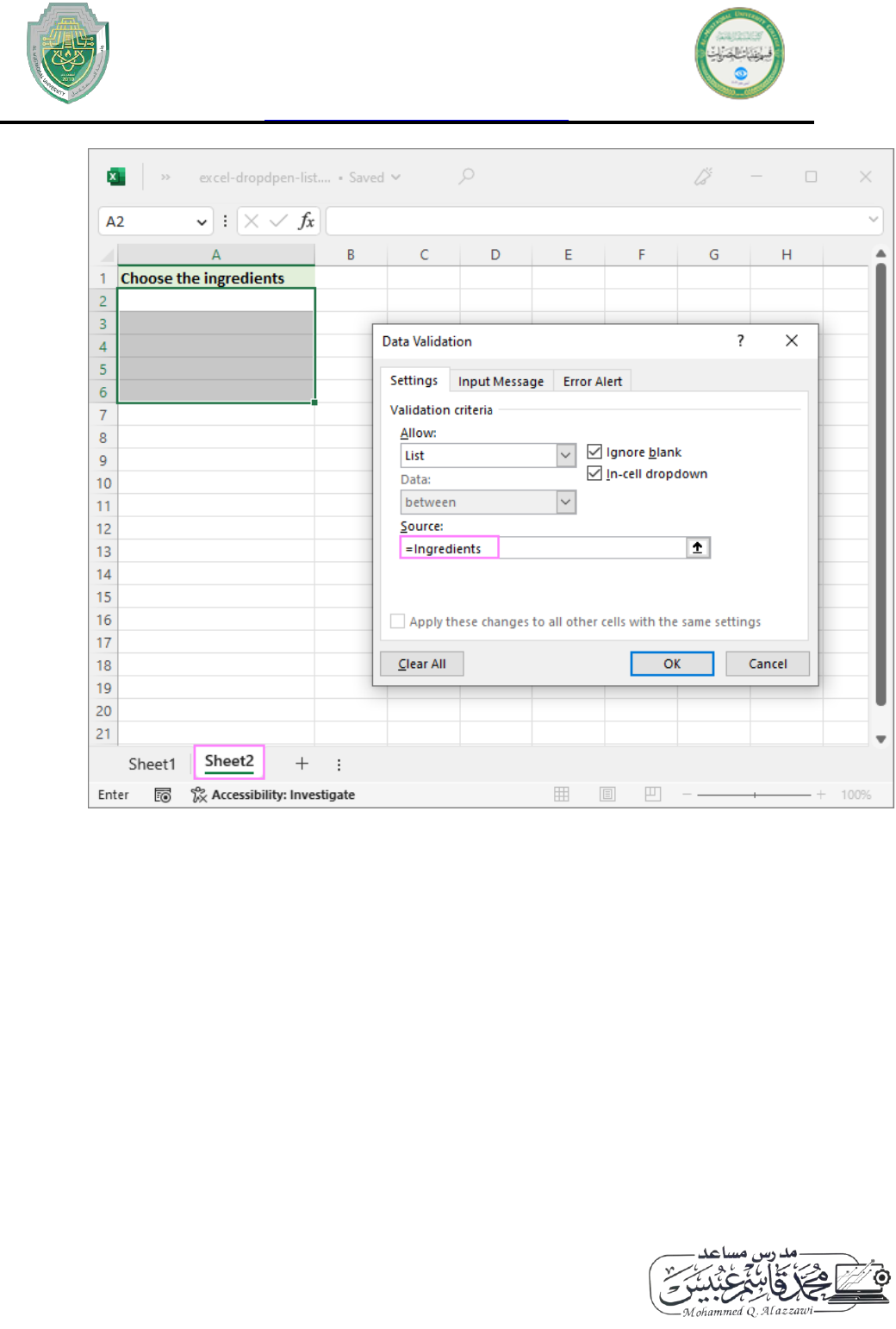
As an example, let's create a range named Ingredients:
3. Select the cells for the picklist - on the same sheet as the named range or
in a different worksheet.
4. Open the Data Validation dialog window and configure the rule:
o In the Allow box, select List.
o In the Source box, type an equals sign followed by the range name.
In our case, it's =Ingredients.
o Click OK.
Al-Mustaqbal University
College of Health and Medical Technologies
Lecturer Mohammed Qasim Al Azzawi
mohammed.[email protected]
Page 7 of 23
Note. If your named range has at least one blank cell, leaving the Ignore blank box
selected allows typing any value in the validated cell.
Advantages: If you insert multiple drop-downs in different sheets, named ranges will
make them a lot easier to identify and manage.
Drawbacks: Takes a bit more time to set up.
Create drop-down from Excel table
Instead of using a named range, you can place the source data into a fully
functional Excel table. Why may you want to use a table? First and foremost,

Al-Mustaqbal University
College of Health and Medical Technologies
Lecturer Mohammed Qasim Al Azzawi
mohammed.[email protected]
Page 8 of 23
because it lets you create an expandable dynamic drop-down list that updates
automatically as you add or remove items to/from the table.
To make a dynamic dropdown from an Excel table, follow these steps:
1. Type the list items in a table or convert an existing range to a table using
the Ctrl + T shortcut.
2. Select the cell(s) where you wish to insert a dropdown.
3. Open the Data Validation dialog window.
4. Select List from the Allow drop-down box.
5. In the Source box, enter the formula referring to a specific column in your
table, not including the header cell. For this, use the INDIRECT function
with a structured reference like this:
=INDIRECT("Table_name[Column_name]")
6. When done, click OK.
For this example, we're making a dropdown menu from the column
named Ingredients in Table1:

Al-Mustaqbal University
College of Health and Medical Technologies
Lecturer Mohammed Qasim Al Azzawi
mohammed.[email protected]
Page 9 of 23
=INDIRECT("Table1[Ingredients]")
Advantages: Easy and quick way to insert an expandable dynamic drop down menu
in Excel.
Drawbacks: Not found :)
How to create a dynamic dropdown list in Excel
If you regularly change the items in your picklist, the best approach is to create
a dynamic drop down list. In this case, the list will update automatically in all the
cells that contain whenever you add or remove items to/from the source list.

Al-Mustaqbal University
College of Health and Medical Technologies
Lecturer Mohammed Qasim Al Azzawi
mohammed.[email protected]
Page 10 of 23
The fastest way to make a dynamic drop down in Excel is from a table as shown
above. That is the default behavior of Excel tables; no extra settings or moves are
required.
Another way is to use a regular named range and reference it with the OFFSET
formula, as explained below.
1. Type the items for the drop down menu in separate cells.
2. Create a named formula. For this, press Ctrl + F3 to open the New
Name dialog box. Type the name you want in the Name box, and then
enter the following formula in the Refers to box.
=OFFSET(Sheet3!$A$2, 0, 0, COUNTA(Sheet3!$A:$A), 1)
Where:
o Sheet3 - the sheet's name
o A - the column where the drop-down items are located
o $A$2 - the cell containing the first item

Al-Mustaqbal University
College of Health and Medical Technologies
Lecturer Mohammed Qasim Al Azzawi
mohammed.[email protected]
Page 11 of 23
3. With the formula name defined, create a dropdown based on a named
range as usual.

Al-Mustaqbal University
College of Health and Medical Technologies
Lecturer Mohammed Qasim Al Azzawi
mohammed.[email protected]
Page 12 of 23
How this formula works
The formula comprises two functions - OFFSET and COUNTA. The COUNTA function
counts all non-blanks in the specified column. OFFSET uses that count for
the height argument, so it returns a reference to a range that includes only non-
empty cells, starting from the cell containing the first item that you supply for
the reference argument.
Advantages: The main advantage of a dynamic drop-down list is that you won't have
to change the reference to the named range each time the source list is expanded
or contracted. You simply delete or type new entries in the source list, and your
dropdown menu will update automatically!
Drawbacks: A bit complex setup process.

Al-Mustaqbal University
College of Health and Medical Technologies
Lecturer Mohammed Qasim Al Azzawi
mohammed.[email protected]
Page 13 of 23
Make a dynamic dropdown list in Excel
Dynamic Array Excel has many innovative functions that are not available in older
versions. One of these new functions named UNIQUE can help you create a
dynamic drop-down with a simple formula.
Suppose you have a dataset with many repeated items like in column A in the
image below. You aim to add a dropdown list where each item appears just once.
To extract the unique items, use this formula:
=UNIQUE(A2:A21)
Optionally, you can sort the extracted values alphabetically by wrapping it in
the SORT function:
=SORT(UNIQUE(A2:A21))

Al-Mustaqbal University
College of Health and Medical Technologies
Lecturer Mohammed Qasim Al Azzawi
mohammed.[email protected]
Page 14 of 23
This dynamic array formula is entered just in one cell (E2) and it
automatically spills into as many cells as needed to show all the unique items.
Next, you set up a drop down list using a spill range reference, which is a cell
address followed by a hash character. In our case it's =$E$2# or =Sheet1!$E$2# if a

Al-Mustaqbal University
College of Health and Medical Technologies
Lecturer Mohammed Qasim Al Azzawi
mohammed.[email protected]
Page 15 of 23
dropdown is in another sheet:
The result is an expandable dynamic drop-down list - the UNIQUE function
automatically extracts new items as they are added to the source table, and the
spill range reference forces Excel to update the drop-down list accordingly.
Tip. The same approach can be used to create a cascading drop-down list in Excel
365. For full details, please see Make a dynamic dependent dropdown list an easy
way.
How to create drop down list from another sheet
To insert a drop-down menu that pulls data from a different worksheet, you can
use a normal range, named range or Excel table:
• When making a dropdown menu from a named range, make sure the scope
of the name is Workbook, and then set up a data validation list as usual.

Al-Mustaqbal University
College of Health and Medical Technologies
Lecturer Mohammed Qasim Al Azzawi
mohammed.[email protected]
Page 16 of 23
• When creating a drop down list from a table, no extra steps are needed as
table names/references are valid across the entire workbook.
• If you insert a drop down from a regular range, include the sheet's name in
the source reference. In the Data Validation dialog window, place the cursor
in the Source box, switch to the other sheet and select the range containing
the items. Excel will add the sheet name to the reference automatically.
How to make drop-down list from another workbook
To create a drop-down menu in Excel using a list from another workbook as the
source, you will have to define 2 named ranges - one in the source workbook and
the other in the workbook where you wish to insert your Data Validation list. The
steps are:

Al-Mustaqbal University
College of Health and Medical Technologies
Lecturer Mohammed Qasim Al Azzawi
mohammed.[email protected]
Page 17 of 23
1. In the source workbook, create a named range for the source list,
say Source_list.
2. In the main workbook, define a name that references your source list. For
this example, we create the name Items that refers to:
=SourceFile.xlsx!Source_list
If the workbook's name contains spaces or non-alphabetical characters, it
must be enclosed in single quotation marks like this:
='Source File.xlsx'!Source_list
For more details, please see How to make external reference in Excel.

Al-Mustaqbal University
College of Health and Medical Technologies
Lecturer Mohammed Qasim Al Azzawi
mohammed.[email protected]
Page 18 of 23
3. In the main workbook, select the cell(s) for your picklist and click the Data
tab > Data Validation. In the Source box, reference the name you created in
step 2. In our case, it's =Items.
Notes:

Al-Mustaqbal University
College of Health and Medical Technologies
Lecturer Mohammed Qasim Al Azzawi
mohammed.[email protected]
Page 19 of 23
• For the drop-down list from another workbook to work, the source workbook
must be open.
• The dropdown list created in this way won't update automatically when items
are added to or removed from the source list - you will have to modify the
source list reference manually.
How to make a dynamic dropdown from another workbook
To create a dynamic dropdown list from another workbook, define a formula
name in the source workbook using the OFFSET formula explained in Creating a
dynamic drop-down in Excel. In this case, a dropdown menu in another workbook
will be updated on the fly once any changes are made to the source list.
Searchable drop down list in Excel
In Excel 365, data validation lists have an awesome AutoComplete feature. To
speed up data entry in large lists, just start typing the target word in the dropdown
menu cell - the autocomplete algorithm will match the typed substring with the
dropdown list items and show you the found matches. As you type more
characters, the displayed list is narrowed down, and conversely, when you remove
characters, more matches are shown.

Al-Mustaqbal University
College of Health and Medical Technologies
Lecturer Mohammed Qasim Al Azzawi
mohammed.[email protected]
Page 20 of 23
Insert a drop down list with message
To show an information message when someone clicks a dropdown list cell,
proceed in this way:
• In the Data Validation dialog box, switch to the Input Message tab.
• Make sure the Show input message when cell is selected option is checked.
• Type the title and message in the corresponding fields (up to 225 characters).
• Click OK to save the message and close the dialog.

Al-Mustaqbal University
College of Health and Medical Technologies
Lecturer Mohammed Qasim Al Azzawi
mohammed.[email protected]
Page 21 of 23
The resulting drop down list with message will look similar to this:
Make an editable drop down list in Excel
By default, an Excel drop-down is non-editable, i.e. restricted to the values in the list
itself. If you type any other value, an error alert will show up. However, you can
allow users to enter their own values. Here's how:
1. Open the Data Validation dialog window.

Al-Mustaqbal University
College of Health and Medical Technologies
Lecturer Mohammed Qasim Al Azzawi
mohammed.[email protected]
Page 22 of 23
2. On the Error Alert tab, uncheck the Show error alert after invalid data is
entered box.
Technically, this turns a drop-down list into a combo box. The term "combo box"
means an editable dropdown that allows users to either select a value from the
predefined list or type a custom value directly in the box.
Optionally, you can display a warning message when someone attempts to enter a
value that is not in the list:
1. On the Error Alert tab, select the Show error alert after invalid data is
entered option.
2. From the Style box, pick either Information or Warning, and then type the
title and message text.
o Information message is best to be used if there is nothing wrong
with the user entering a custom value.
o Warning message will induce users to select an item from the drop-
down box rather than enter their own data, though it does not
prohibit it.

Al-Mustaqbal University
College of Health and Medical Technologies
Lecturer Mohammed Qasim Al Azzawi
mohammed.[email protected]
Page 23 of 23
And here's an editable Excel dropdown list with a warning message in action:
